Hillslope Delineation and Critical Duration Tools

March 2022

tip

Download the PDF here

Executive Summary

Summary of document

The Arc Hydro Hillslope and Critical Duration tools are automated geoprocessing tools created through original research at the University of California, Berkeley. These tools delineate hillslopes, fit exponential HWFs to the delineated hillslopes, and assess the degree to which curvature may impact hydrological model predictions (using the Rational Method as an illustrative example). The Hillslope and Critical Duration toolset is available in ArcGIS Pro 2.7 and higher as part of the Arc Hydro Pro add-in. This document describes the implementation of Hillslope and Critical Duration tools within the Arc Hydro Pro framework. This includes:

• Getting started with Hillslope and Critical Duration tools (example datasets)

• Overview of tools with descriptions of input and output parameters, and example runs

  • Pre-requisite tools

  • Hillslope tools

  • Critical Duration tools

• Appendix that includes more detail on tool processes, user-defined input parameters, and IDF curve parameter estimation

For additional detail on and use cases for the Arc Hydro Hillslope and Critical Duration tools, see publication by Lapides and Sytsma et al. 2022.

Document history

Table 1. Document Revision History

Version	Description	Date
1	Initial document (AS & GLO).	March 2022

Getting started with Hillslope and Critical Duration Tools

Arc Hydro Hillslope and Critical Duration tools are included in the installation of Arc Hydro Pro.

• Guidelines for installing Arc Hydro are available from: https://community.esri.com/t5/water-resources-questions/arc-hydro-installation-versions-and-documentation/m-p/269522

• Users should install version 2.9.24 or higher of Arc Hydro from: http://downloads.esri.com/archydro/ArcHydro/Setup/Pro/.

• Testing data used in this documentation can be found under "Hillslope_data" here: http://downloads.esri.com/archydro/archydro/Tutorial/Data/.

Toolset overview

Intended Workflow

The Hillslope and Critical Duration tools are intended to be used as part of the following workflow:

1. A digital elevation model (DEM) is prepared for hydrologic analysis by applying hydroconditioning such as Fill (optional) and basic terrain processing. The results of this DEM preparation should include: a flow accumulation raster, a flow direction raster, drainage lines (or streams), watersheds, and a corresponding flow accumulation threshold that was used to generate the streams.

2. Watersheds for the area of interest are partitioned into headwater hillslopes (draining to a stream initiation point) and lateral hillslopes (draining to a stream reach forming the hillslope's lower boundary).

3. Hillslope shapes are approximated with an exponential hillslope width function.

4. Hillslope roughness is estimated using landcover information.

5. The hillslopes, with estimated parameters for shape and roughness, are used to estimate the time of concentration and the critical duration for a user-defined return interval storm.

6. Storm event hydrographs for the user-defined return interval storm are generated.

The Hillslope and Critical Duration tools execute steps 1-5, implemented as Arc Hydro python tools. The tools are split between two toolboxes (Figure 1).

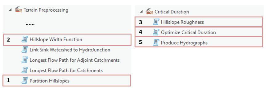
Figure 1. Arc Hydro Pro toolset implementation of the Hillslope and Critical Duration tools, where the ordering represents the intended order of use

The "Terrain Preprocessing" toolbox contains: (1) the Hillslope Partitioning tool, which delineates hillslope areas; and (2) the Hillslope Width Function tool, which fits the hillslopes with an exponential hillslope width function (HWF).

The "Critical Duration" toolbox contains: (3) the Hillslope Roughness tool, which computes the roughness term needed for peak flow calculation; (4) the Optimize Critical Duration tool, which uses overland flow theory to compute the impact of hillslope curvature on peak flow predictions; and (5) the Produce Hydrograph tool, which produces a storm hydrograph for a user-defined rainfall duration and intensity.

Data requirements and conventions

Required input data are a high-resolution digital elevation model (DEM) and a land cover raster from the National Land Cover Database (NLCD). The input data must adhere to Arc Hydro data requirements:

• Rasters are in an Esri supported raster format; TIFF is recommended.

• Horizonal and vertical units for raster and vector/tabular data will be in consistent units (ft or m) and projection.

All vector data created with the Hillslope and Critical Duration tools will be saved to the default project geodatabase, within a "Layers" feature dataset that will be automatically created. The output data will be in the projection matching the projection of the DEM.

Example input data structures

The following figures represent a valid sample dataset.

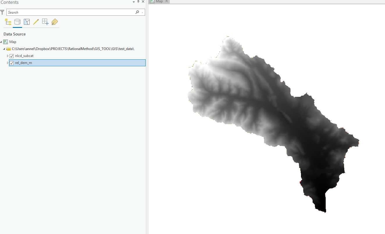
Figure 2. Example DEM from the Arc Hydro Hillslope and Critical Duration tool test data.

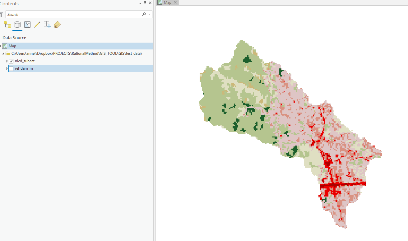
Figure 3. Example land cover raster from the Arc Hydro Hillslope and Critical Duration tool test data.

The map contains:

1. DEM ("rel_dem_m"). Note that the DEM structure controls the raster outputs for the following parameters:

   1. Raster format (e.g., if DEM is in TIFF format, all the outputs will be in TIFF).

   2. Cell size.

   3. Analysis extent.

2. Land cover raster ("nlcd_subcat"). The land cover raster must have land covers classified in accordance with NLCD classification. See Appendix Section 4.2 for additional detail.

Value	Class names
11	Open water
21	Developed, open space
22	Developed, low intensity
23	Developed, medium intensity
24	Developed, high intensity
31	Barren land
41	Deciduous forest
42	Evergreen forest
43	Mixed forest
52	Shrub/scrub
71	Grassland/herbaceous
81	Pasture/hay
82	Cultivated crops
90	Woody wetlands
95	Emergent herbaceous wetlands

Output data structures & naming conventions

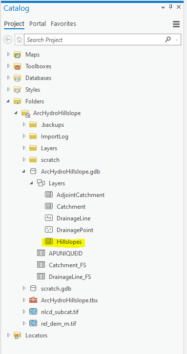
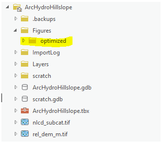
Tools create numerous output data structures. To ensure consistency of application and result data, all the results are placed in predetermined data and naming structure with minimal user input. All created outputs will be stored in the Project Folder (Figure 4) by default. Raster outputs will be saved to a child directory, "Layers". Vector and tabular outputs will be saved to the project geodatabase ("ArcHydroHillslope.gdb" in Figure 4). More specifically, vector data will be saved to the "Layers" feature dataset of this geodatabase. Default output naming conventions are in place as a convenience to users, however these can be changed to custom names and locations if desired.

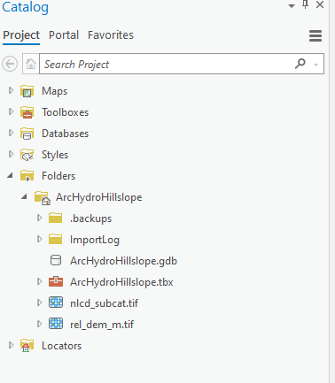
Figure 4. Example file structure. Here, the input test data ("nlcd_subcat" and "rel_dem_m") have been imported to the project folder.

The following sections present operation for the five Arc Hydro Hillslope and Critical Duration tools. Screenshots of the tools include parameters that correspond to the example dataset provided (see Section 2.0).

Pre-requisite tools

This section describes two pre-requisite Arc Hydro tools to use prior to the Hillslope and Critical Duration tools.

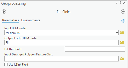
Fill Sinks (Optional)

This tool is used to fill sinks present in the original DEM. Arc Hydro documentation provides more details on sink screening.

For the test data provided here, we use the Fill Sinks on the input DEM ('rel_dem_m') and use default parameters and output ('Fil').

Terrain Preprocessing

The Terrain Preprocessing tools include terrain preprocessing workflows for deranged, combined, and dendritic terrains. Arc Hydro documentation provides further details on the Terrain Preprocessing tools.

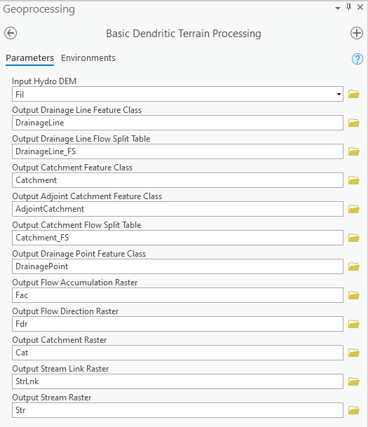For the test data provided here, we use the Basic Dendritic Terrain Processing tool, which is appropriate for terrain with no sinks, only streams. The filled DEM described above is used as input (see Figure below).

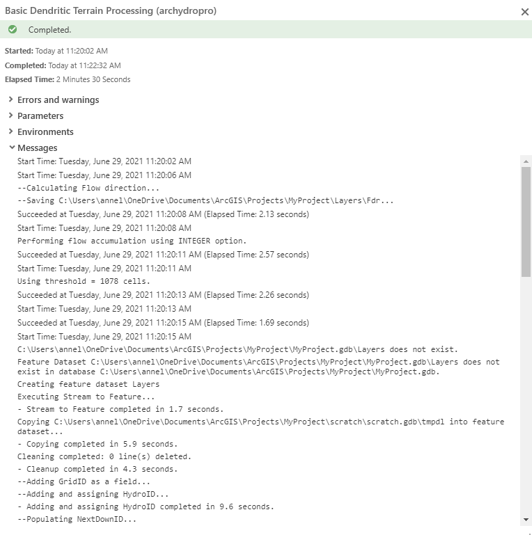
After running the Basic Dendritic Terrain Processing tool, the flow accumulation threshold can be found by examining the "messages" (see Figure below). For the test data provided, this threshold is 1078 cells. This information is needed for the hillslope partitioning step.

Hillslope Tools

The following sections describe the tools used to delineate hillslopes and calculate hillslope width functions. Screenshots of the tools include parameters that correspond to the example dataset provided (see Section 2.0).

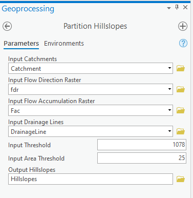
Partition Hillslopes

Separate subwatersheds into headwater and lateral hillslopes. Headwater hillslopes drain to stream inlets and lateral hillslopes are created by bisecting the relevant catchment area by the drainage line. Hillslope parts that are the size of the user defined area threshold or smaller are deleted from the final output.

An example of the Partition Hillslopes tool is shown below. Inputs correspond to the example dataset provided (See Section 2.0) and build on the outputs of the Terrain Preprocessing Tool (Section 3.3.1). Default naming was used for the output hillslope feature layer, with the default output folder.

1. Tool parameters

   Input Catchments

   Input catchment feature layer following the Arc Hydro data model.

   Input Flow Direction Raster

   Input flow direction raster following the Arc Hydro data model.

   Input Flow Accumulation Raster

   Input flow accumulation raster following the Arc Hydro data model.

   Input Drainage Lines

   Input drainage lines following the Arc Hydro data model.

   Input Threshold Number of cells used as the flow accumulation threshold when creating the drainage lines. This number is used to identify stream inlets. See the user messages for the flow accumulation threshold used in terrain preprocessing steps.

   Input Area Threshold

   Minimum hillslope area to retain in output.

   Output Hillslopes Output hillslope feature class. Any hillslope parts are the size of one cell or smaller are deleted.

2. Example run

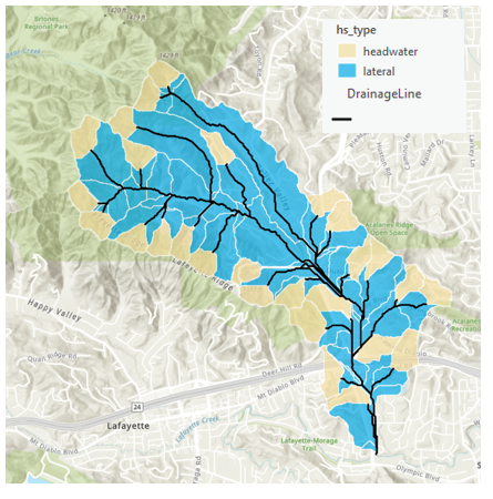
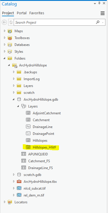
The following data structures were created as a result of the tool run (left, highlighted in yellow). The following map (right) is an example output of this step, showing delineated hillslopes with unique symbology by the field "hs_type".

Hillslope Width Function

Fits each hillslope with a best-fit exponential hillslope width function of the form:

where W is the width of the hillslope and x is the distance from the hillslope divide. The resulting exponential hillslope conserves the area of the original hillslope by modifying the hillslope length. The following error metrics are calculated:

• shape_err: Higher values mean a better fit between observed hillslope widths and the widths predicted by the HWF.

• pt_err: Larger values imply a poor approximation of the hillslope by the points. This can be improved by increasing the number of points used.

• pt_trunc_err: Larger values imply large truncation of hillslope area needed to satisfy assumption of monotonic hillslopes.

• strm_err (lateral hillslopes only): Larger values mean that the approximation of linear stream channel may not be valid.

This tool modifies the input hillslopes feature with new fields: 'a', 'c', 'xend', 'xtop', 'L', 'shape_err', 'pt_err', 'pt_trunc_err',and 'strm_err'.

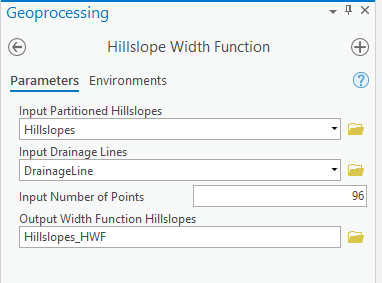
An example of the Hillslope Width Function tool is shown below. Inputs correspond to the example dataset provided (See Section 2.0) and build on the outputs of the Partition Hillslopes Tool (Section 3.4.0). Note that we use 96 for the input number of points, but any integer between 4 and 100 is valid.

1. Tool parameters

   Input Partitioned Hillslopes
   
       Input partitioned hillslopes (use "Partition Hillslope" tool in Terrain

   Preprocessing).

   Input Drainage Lines
   
       Input drainage lines following the Arc Hydro data model.
   
   Input Number of Points
   
       Number of points to approximate the hillslope (must be an integer between 4 and 100).
   
   Output Width Function Hillslope
   
       Output hillslopes with width function applied (default name: "Hillslopes\_HWF")

2. Example run

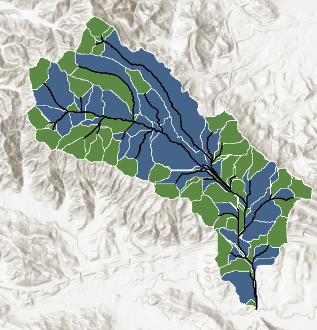
The following data structures were created as a result of the tool run (left, highlighted in yellow). The following map (right) is an example output of this step, showing delineated hillslopes with a < 0 (convergent hillslopes) and a > 0 (divergent hillsopes).

Critical duration tools

The following sections describe the tools used to calculate the Critical Duration for hillslopes in a catchment.

Hillslope Roughness

The kinematic roughness equations require a roughness parameter alpha, given by:

where S is slope [L/L] and n is Manning's roughness coefficient. This step computes the mean hillslope slope S, the area-weighted Manning's roughness coefficient n, and uses these to compute alpha.

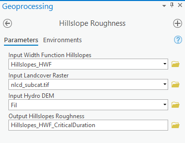
An example of the Hillslope Roughness tool is shown below. Inputs correspond to the example dataset provided (See Section 2.0) and build on the outputs of the Hillslope Width Function Tool (Section 3.4.1).

1. Tool parameters

   Input Width Function Hillslopes

   Partitioned hillslopes with hillslope width function attributes calculated using the Hillslope Width Function tool (Terrain Preprocessing).

   Input Landcover Raster

   Input NLCD landcover raster. See <https://www.mrlc.gov/>.

   Input Hydro DEM

   Input Filled DEM following the Arc Hydro data model.

   Output Hillslopes Roughness

   Output hillslopes with *alpha* calculated.

2. Example run

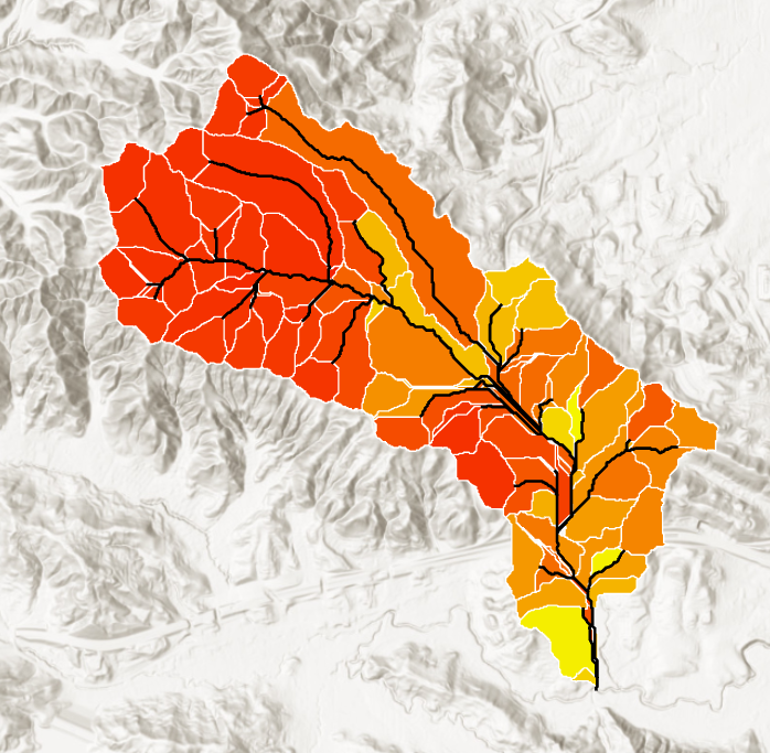
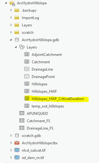
The following data structures were created as a result of the tool run (left, highlighted in yellow). The following map (right) is an example output of this step, showing delineated hillslopes with alpha in graduated colors.

Optimize Critical Duration

Simulates overland flow across each hillslope using analytical solution, calculates dcrit (critical duration, or duration of storm that produces peak discharge), tc (time that the entire hillslope contributes to flow at the outlet), Qmax (peak flow for the return interval at dcrit), Amax (maximum contributing area for the return interval), C_calc (calculated runoff coefficient at Qmax and dcrit), Qtc (flow corresponding to tc), and ratio of dcrit to tc (dc_tc). In cases where tc is never reached, the ratio dc_tc will be NA, and dcrit will by definition be less than tc. When dcrit < tc, the field dc_lt_tc is YES, otherwise it is NO. This tool modifies the input hillslopes feature with the newly calculated fields added.

An example of the Optimize Critical Duration tool is shown below. Inputs correspond to the example dataset provided (See Section 2.0) and build on the outputs of the Hillslope Roughness Tool (Section 3.5.0).

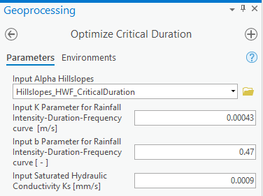
1. Tool parameters

   Input Alpha Hillslopes

Partitioned hillslopes with alpha calculated using Hillslope Roughness tool.

Input K Parameter for Rainfall Intensity-Duration-Frequency Curve

Input K from intensity-duration-frequency curve function of the form: I=K/(D^b) (typical values range from 0.0001 to 0.001 m/s).

Input b Parameter for Rainfall Intensity-Duration-Frequency Curve

Input b from intensity-duration-frequency curve function of the form: I=K/(D^b) (typical values range from 0.4 to 0.65).

Input Saturated Hydraulic Conductivity Ks

Input approximation for saturated hydraulic conductivity in mm/s. This is subtracted from the intensity to give an effective rainfall rate.

For refence, sandy loam soil Ks ~ 0.008 mm/s, loamy soil Ks ~ 0.0009 mm/s, and clay soil Ks ~ 0.00008 mm/s (Rawls et al. 1983)

2. Example run

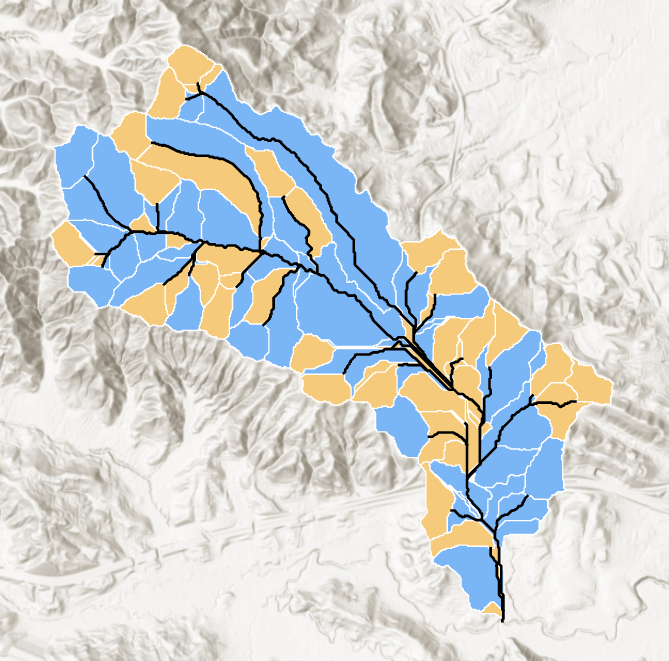
The following data structures were created as a result of the tool run (left, highlighted in yellow). The following map is an example output of this step, showing delineated hillslopes with colors corresponding to dc_lt_tc = YES (where dcrit < tc and using tc underestimates Qmax) and dc_lt_tc = NO (where dcrit = tc).

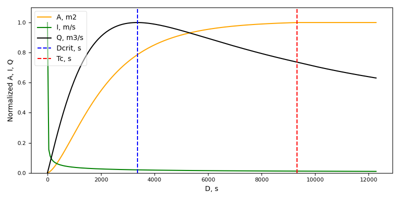
The "Figures/optimized" folder contains plots of the optimized hillslope hydrographs, with the suffix of the resulting figure name given by the "FID_hillsl" field. An example output is shown below for a divergent hillslope ('optimized_24'), where dcrit < tc. The x-axis shows duration (s) and the y-axis shows normalized A(D), I(D), and Q(D) values.

Produce Hydrographs

Calculates the peak flow (Q_max_tr, in m3/s) for each hillslope using the IFD curve parameters K and b, saturated hydraulic conductivity Ks, and critical duration dcrit (from Optimize Critical Duration tool) for user-defined storm duration tr (s). This tool modifies the input hillslopes feature with new fields: tr, I, and Q_max_tr. This tool also produces hydrographs for each hillslope in a 'Figures/hydrograph' folder in the parent directory of the input hillslopes feature.

An example of the Produce Hydrograph tool is shown below. Inputs correspond to the example dataset provided (See Section 2.0) and build on the outputs of the Optimize Critical Duration tool (Section 3.5.1).

1. Tool parameters

   Input Optimized Hillslopes Partitioned hillslopes with hillslope optimization (output of "Optimize Critical Duration" tool).

   Input storm duration (s)

   Input duration of storm event in s.

2. Example run

The following data structures were created as a result of the tool run (highlighted in yellow).

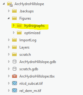
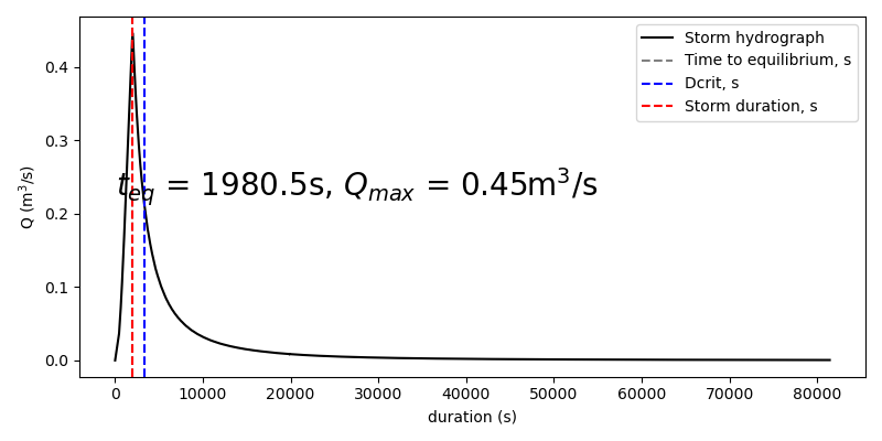The "Figures/hydrograph" folder contains plots of the hillslope hydrographs for the single storm specified, with the suffix of the resulting figure name given by the "FID_hillsl" field. An example output is shown below for a single hillslope ('hydrograph_24'). The x-axis shows duration (s) and the y-axis represents Q (m3/s).

Appendix

Tool processes

This section provides a more in-depth description of the processes involved in each tool. For additional detail, refer to the scripts in the Arc Hydro toolbox.

Partition Hillslopes

This tool identifies stream inlet points and delineates catchments draining to stream inlet points to give headwater hillslopes. This process involves delineating full catchments, mosaicking headwater and full catchments, and bisecting with stream channel to give lateral hillslopes.

The tool performs the following actions:

1. Delineates headwater catchments

   • Identifies threshold points using the Identify Threshold Points Arc Hydro tool. This tool utilizes the flow direction raster, flow accumulation raster, and threshold integer inputs.

   • Delineates catchments draining to the threshold points using the Spatial Analyst Watershed tool, leaving the headwater catchments delineated in raster format.

   • Converts the headwater catchments raster to polygon format.

2. Bisects lateral hillslopes

   • Isolates conjoined lateral hillslopes by erasing headwater catchments from the full catchments input feature.

   • Extends the drainage lines input feature by 50 units to ensure each conjoined lateral hillslope is fully bisected by drainage lines.

   • Uses arcpy Geometry operations to (1) select the geometry of each conjoined lateral hillslope and its intersecting drainage line, and (2) cut the hillslope by the line. This returns lateral hillslopes as a left and right part of the conjoined lateral hillslope.

   • Combines headwater and full watersheds.

   • Combines headwater and lateral hillslopes into a single feature class and attribute as necessary.

   • Removes any catchments that are smaller than the Input Area Threshold parameter.

Hillslope Width Function

This tool fits each hillslope delineated with a best-fit exponential hillslope width function of the form:

where W is the width of the hillslope, x is the distance from the hillslope divide, c parameterizes width at the divide, and a determines the degree and nature of hillslope curvature. When a > 0, the hillslope is divergent, and when a < 0, the hillslope is convergent, and a = 0 describes a uniform-width hillslope.

A hillslope width function (HWF) represents the topographic shape of a hillslope. We denote a line from the divide of a hillslope to the outlet as the x-axis. At each value x along the hillslope, the width w(x) represents the linear distance between contour endpoints. This definition requires reconciliation of actual hillslopes with idealized exponential hillslope shapes. We applied two criteria to the process of delineating hillslope width functions, following Noel et al. (2014): (1) monotonicity and (2) conservation of area. Monotonicity ensures that the hillslope width function is convergent (monotonically increasing), divergent (monotonically decreasing), or constant (uniform), while conservation of area fulfills mass conservation requirements.

The tool performs the following actions:

1. Points along hillslope boundary

   • Hillslopes are converted to polylines and the stream network is erased from the polyline, resulting in hillslope outlines with a discontinuity at the outlet location.

   • Two points were generated along the hillslope outlet ("outlet points"), placed at either endpoint of the discontinuity, and a line was formed from these two points ("outlet line").

   • j equally spaced points are generated along the hillslope polyline ("hillslope points"). Any integer between 4 and 100 is a valid entry for this parameter.

2. Pair points across midline

   • Next, the j hillslope points are paired with the corresponding point across the hillslope, and a midline is drawn up the vertical axis of the hillslope, given by the best fit line for the midpoints of each point pair. This midline is the x-axis for defining the HWF.

   • The midline separates the hillslope points into points to the left and right of the midline.

3. Compute W and x for each hillslope point pair

   • For each point on the right, the perpendicular distance to the midline is the width of the right half, and the perpendicular distance to the outlet is used to find the position along the x-axis as a distance from the divide.

4. Hillslope width function

   • From these paired distances and widths, the tool calculates the parameters c and a, which provide the optimal best fit for the right side of the hillslope. The same is done for the left side of the hillslope.

   • An overall exponential fit is found by calculating the exponential function which equates to the sum of the left and right sides to calculate final values of c and a.

5. Area conservation

   • To ensure that area is conserved in the exponential fit, we keep the location of the outlet (to maintain the same outlet width) and calculate the location of the divide that preserves the area of original hillslope.

   • Using the x-location of the hillslopes divide (x_0) and outlet (x_end) and the exponential best fit parameters for c and a, we fully describe the exponential HWF.

6. Error metrics

   • 'pt_err': percent error between the actual hillslope area and the polygon constrained by the hillslope points and outlet points. Larger pt_error implies a poor approximation of the hillslope by the points, and can be improved by increasing the number of points used. computed as the percent error between the actual hillslope area and the polygon area constrained by the hillslope points and outlet points. This metric is indicative of the degree to which the points chosen represent the hillslope shape. If the area bounded by the points is not representative of the shape or area of the original hillslope, the point selection error will be large.

   • 'shape_err': R² value (ranges from 0 to 1) between observed hillslope widths and the widths predicted by the HWF (higher shape_err means a better fit).

   • 'pt_trunc_err'. percent error between polygon constrained by the hillslope points and outlet points and hillslope defined by truncated points. Points are truncated where hillslope stops increasing or decreasing in width (to satisfy assumption that hillslopes are increasing or decreasing monotonically). Larger pt_trunc_err means that a large portion of the hillslope was truncated in this process.

   • 'strm_err' (for lateral hillslopes only): percent error between the Euclidean stream distance (measured as the linear distance between lateral hillslope outlet points) and the actual stream distance. Larger strm_err values mean that the approximation of linear stream channel may not be valid.

Hillslope Roughness

This tool computes hillslope roughness coefficient (alpha) from slope (S) and manning's roughness coefficient (n). Manning's roughness coefficient is estimated from land cover data from the National Land Cover Database. The output is a hillslope feature layer with field containing area-weighted alpha value.

The tool performs the following actions:

1. Computes slope

   • Computes pointwise slope from the input DEM, averages over the hillslope area to give the average hillslope slope S.

2. Computes Manning's roughness coefficient

   • Converts land cover raster from NLCD to n using a look up table developed by Kalyanapu (2009) (see table below).

   • Computes area weighted n for each hillslope.

   • Alternatively, if an NLCD landcover dataset is not available (e.g., if the tool is applied outside of the United States), the use can provide any land cover raster with values that match the NLCD land cover categories. See the Appendix Section 4.2 for additional guidance for this approach.

3. Computes for each hillslope.

VALUE	class names	Manning's n
11	Open water	0.001
21	Developed, open space	0.0404
22	Developed, low intensity	0.0678
23	Developed, medium intensity	0.0678
24	Developed, high intensity	0.0404
31	Barren land	0.0113
41	Deciduous forest	0.36
42	Evergreen forest	0.32
43	Mixed forest	0.4
52	Shrub/scrub	0.4
71	Grassland/herbaceous	0.368
81	Pasture/hay	0.325
82	Cultivated crops	0.037
90	Woody wetlands	0.086
95	Emergent herbaceous wetlands	0.1825

Optimize Critical Duration

This tool performs a numerical optimization by calculating the values of A(D), Q(D), and C(D)=Q/AI for a range of storm durations using the analytical solutions for user-defined IFD constants K (m/s) and b and user-defined soil saturated hydraulic conductivity Ks (mm/s).

The user defined soil saturated hydraulic conductivity Ks are catchment specific; values for this may be found in local watershed reports or national databases (e.g., the Web Soil Survey). For refence, sandy loam soil Ks ~ 0.008 mm/s, loamy soil Ks ~ 0.0009 mm/s, and clay soil Ks ~ 0.00008 mm/s (Rawls et al. 1983).

This tool calculates D_crit (time of max flow), Tc (time that the entire hillslope contributes to flow at the outlet), Qmax (peak flow for the return interval), and ratio D_crit/Tc. This tool also produces plots of the optimization results for each hillslope in a 'figures/optimized' folder in the parent directory of the input hillslopes feature.

The tool performs the following actions:

1. Computes effective rainfall rate, I

   • For each storm duration D, calculates an effective raintall rate (Rational Method parameter I) using the equation:

     

   • K and b are the IFD curve parameters and the saturated hydraulic conductivity Ks represents a constant loss rate.

2. Computes overland flow, Q

   • For each storm duration and hillslope, calculates flow Q using analytical solutions (see Lapides et al. 2020) for overland flow on hillslopes represented by a HWF with parameters c, a, xtop0, and xend.

   • HWF parameters provided as fields in the Input Alpha Hillslopes feature class.

3. Computes runoff coefficient, C

   • For each storm duration and hillslope, calculates C from the Rational Method relationship:

4. Computes critical duration, Dcrit

   • For each hillslope, finds the storm duration dcrit for which Q = CIA is maximized.

   • Computes the corresponding flow ("Qmax") and area ("Amax") at dcrit_.

5. Computes the time of concentration, tc.

   • For each hillslope, finds the first storm duration tc for which the entire hillslope area is contributing to flow at the outlet .

   • Computes the corresponding flow at tc ("Qtc").

6. Computes comparison metrics

   • For each hillslope, computes the ratio of dcrit to tc ("dc_tc"). In cases where tc is never reached, the ratio dc_tc will be NA, and dcrit will by definition be less than tc.

   • When dcrit is less than tc, a field "dc_lt_tc" is YES, otherwise it is NO.

Produce Hydrographs

This tool calculates the peak flow (cms) for each hillslope with user-defined values of storm duration tr (s) and storm intensity i (m/s). This step assumes the same user-defined soil saturated hydraulic conductivity Ks as specified in the Optimize Critical Duration Tool.

This tool adds the following fields:tr(input storm duration), i (computed storm intensity), and Q_max_tr (calculated peak flow in cms corresponding to tr and i), and also produces hydrographs for each hillslope in a 'figures/hydrographs' folder in the parent directory of the input hillslopes feature.

The tool performs the following actions:

1. For each hillslope, calculates the effective rainfall rate i using the input duration (tr), and previously specified values for the IDF curve (K, b) and K using the equation:

   

2. For the storm defined by the duration (tr) and effective rainfall rate, calculates the peak flow Q_max_tr using analytical solutions (see Lapides et al. 2020) for overland flow on hillslopes represented by a HWF with parameters c, a, xtop0, and xend (provided as fields in the input feature class).

3. Plots the resulting storm flow hydrograph.

Using user-defined land cover or roughness values

If an NLCD landcover dataset is not available or if the tool is applied outside of the United States, the user can use any land cover raster with values that match the NLCD land cover categories. For example, if a user developed their own land cover classification raster with impervious/ urban areas, wetlands, and water classes, these could be re-classified with the NLCD codes below (e.g., using the 'raster reclassification' tool in ArcGIS).

VALUE	class names
11	open water
24	developed, high intensity
95	emergent herbaceous wetlands

It is important, however, that the resulting raster matches NLCD fields: it must contain "VALUE" field that contains the corresponding NLCD "VALUE" code.

If the user wants to supply custom Manning's roughness coefficients directly (rather than estimate based on landuse), they will need to calculate alpha outside of the Arc Hydro environment. Assuming the user has a raster layer with Manning's roughness coefficients specified, the process for this would involve:

• Use the filled DEM to calculate mean slope for each hillslope

• Calculate area weighted roughness coefficient for each hillslope

• Compute alpha for each hillslope as

  where *S* is the mean slope and *n* is the area- weighted manning's roughness coefficient

Estimating IDF Curve Parameters

The IFD constants K and b are based on a power law approximation to an IFD curve (Koutsoyiannis, 1998):

In this approximation, K (in units of m/s) determines how intense storms are for a given return period. Stormier climates and longer return periods have larger values of K, with typical values ranging from 0.0001 to 0.001 m/s.

The constant b is related to rainfall variability, with typical values ranging from 0.4 to 0.65. Smaller values of b are associated with monsoonal, polar, or orographic rainfall patterns, and higher values of b are associated with convective rainfall.

Users can identify values for K and b by fitting equation the power law equation above to regional IFD curves. For example, we determined K and b parameters for the sample data provided in this manual by fitting power law equation above to regional IFD curves for Reliez Creek. For Contra Costa County, CA, where Reliez Creek is located, IFD data are available graphically for different RI storms (5-year RI,10-year RI, 25-year RI, 50-year RI, 100-year RI). For each return interval, we:

• Tabulated by hand the rainfall depth associated with the 508 mm/year (20 inches/year, or the mean annual precipitation for the County) contour for the same storm durations of 5 min, 10 min, 15 min, 30 min, and 1 hr.

• Converted the resulting rainfall depths to average intensities by dividing the depth by its corresponding duration.

• Plotted the duration vs. the average intensity and fitted the points with a power law approximation.

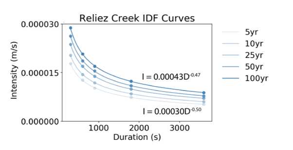The resultant IFD curves are shown in the plot below, with fitted equations shown for the 100 year and 5-year RI storms. The constants in the fitted equation give us values for *K* and *b.*

In the example run shown in Section 3.5.1 (Optimize Critical Duration), we use IFD curve parameters K and b that correspond to the 100-year return interval (RI) storm: K = 0.00043 m/s and

In the example run shown in Section 3.5.2 (Produce Hydrographs), we use these IFD curve parameters K and b to calculate the 100-year storm intensity that corresponds to a storm duration of 2000 s. Note that while any storm intensity and duration can be used in the Produce Hydrographs tool, the critical duration that is plotted on the hydrograph is only relevant for the RI specified in the Optimize Critical Duration tool.

References

• Kalyanapu, A. J., Burian, S. J., & McPherson, T. N. (2009). Effect of land use-based surface roughness on hydrologic model output. Journal of Spatial Hydrology, 9(2), 51-71.

• Koutsoyiannis, D., Kozonis, D., & Manetas, A. (1998). Intensity-Duration-Frequency Relationships. 206, 118-135.

• Lapides, D. A., David, C., Sytsma, A., Dralle, D., & Thompson, S. (2020). Analytical Solutions To Runoff On Hillslopes With Curvature: Numerical And Laboratory Verification. Hydrological Processes, n/a(n/a), hyp.13879. https://doi.org/10.1002/hyp.13879

• Lapides, D., Sytsma, A., O'Neil, G., Djokic, D., Thompson, S.E. (In review at Journal of Environmental Modelling and Software). Arc Hydro Hillslope and Critical Duration: new tools for hillslope hillslope-scale runoff analysis.

• Noel, P., Rousseau, A. N., Paniconi, C., & Nadeau, D. F. (2014). Algorithm for delineating and extracting hillslopes and hillslope width functions from gridded elevation data. Journal of Hydrologic Engineering, 19(2), 365-374. https://doi.org/10.1061/(ASCE)HE.1943-5584.0000783

• Rawls, W. J., Brakensiek, D. L., Miller, N., Asce, M., Brakensiek, D. L., & Miller, N. (1983). GREEN-AMPT INFILTRATION PARAMETERS FROM SOILS DATA. Journal of Hydraulic Engineering, 109(1), 62-70. https://doi.org/10.1061/(ASCE)0733-9429(1983)109:1(62)