Using DSWE for Wetland Identification
Download the PDF here
Introduction
In its baseline implementation, WIM's predictor variables are topographic derivatives, which serve as proxies for near-surface soil moisture. This presents a challenge in areas with low topographic relief and where a complex subsurface exists due to glacial or coastal influence. In these areas, additional information from alternative sensors can improve predictions.
WIM applications in Minnesota have shown the Dynamic Surface Water Extent (DSWE) data product may improve wetland detection for these cases. DSWE is derived from Landsat imagery and is provided by the USGS. Surface water modeled by DSWE provided the ability to include seasonally fluctuating attributes, whereas topographic derivatives model time-averaged wetland characteristics. We also found that DSWE data more accurately captured small waterbodies compared to national-scale hydrography datasets.
Impact of DSWE on WIM Predictions
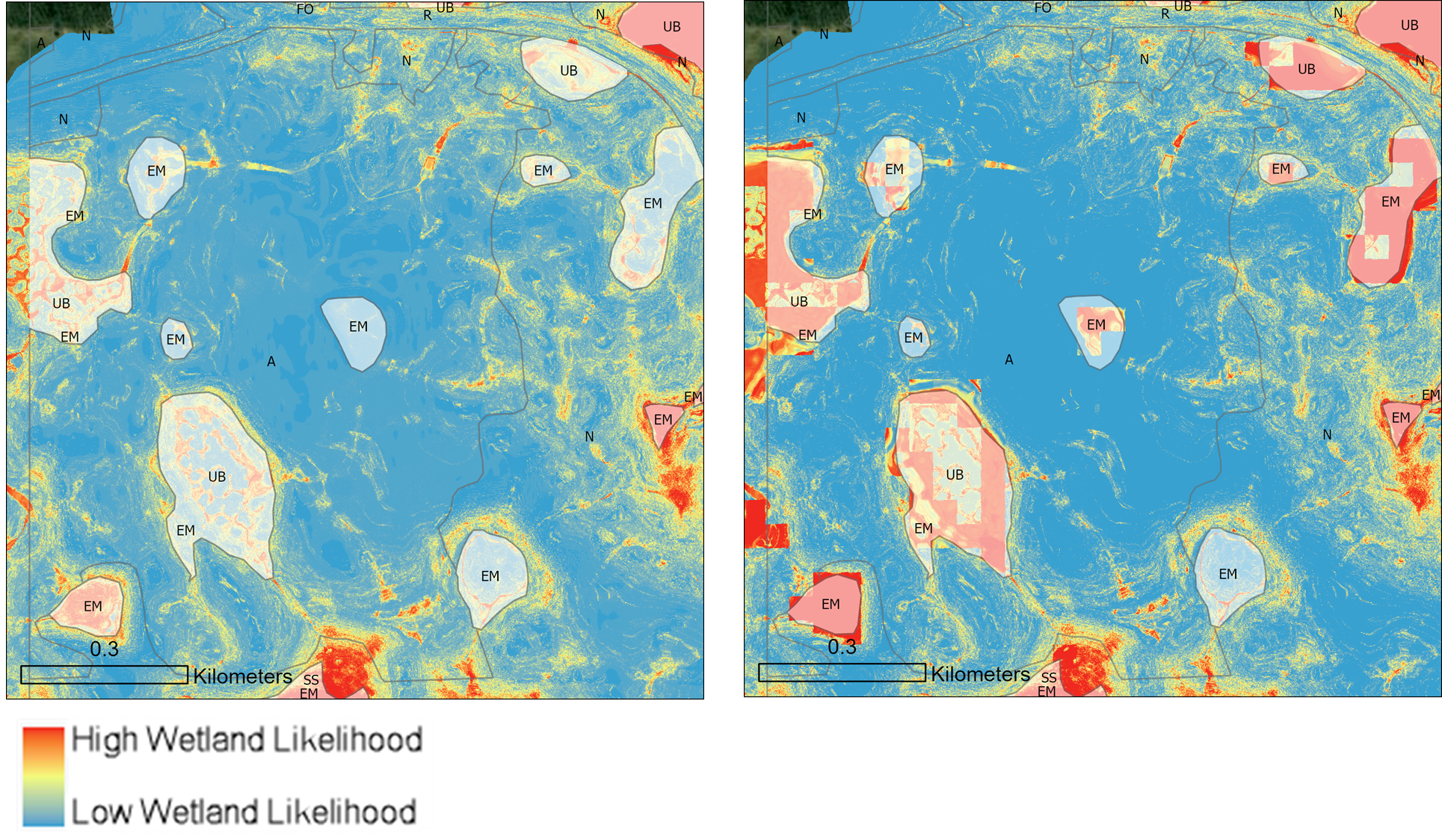
Screenshots below exemplify the impact of DSWE data on wetland predictions for a region in Minnesota. On the left, the WIM model used the baseline topographic inputs as predictor variables. On the right, the WIM model incorporated a May DSWE scene in addition to baseline inputs. In both scenes, ground truth wetlands are shown in white shading, denoted with wetland classes. We can see the WIM model using DSWE captured more of the ground truth wetland area in its predictions. These newly identified wetlands are geographically isolated and disconnected from surface water networks, making them difficult to detect with topographic derivatives alone. The addition of DSWE information also resulted in better areal coverage of wetland likelihood within the larger wetlands.
How to Incorporate DSWE into the WIM Workflow
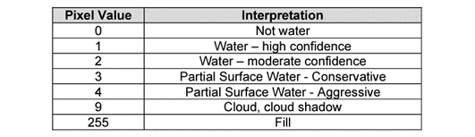
DSWE scenes are available for download from the USGS Earth Explorer (Landsat > Landsat Collection 2 Level-3 Science products > Landsat 4-9 C2 Dynamic Surface Water Extent). Users should select a scene from the season of interest (e.g., early Spring to identify higher wetness potential) and work with the Interpreted Layer with All Masks Applied (INWAM) data product (see more [here]). Values of the INWAM raster represent levels of confidence of surface water presence (see table from DSWE documentation below).
While this raster can be used as a predictor variable directly with WIM, we recommend additional processing. Mainly, we recommend using the DSWE high-confidence areas as part of the surface water input to calculate Depth-to-Water index. This allows the DSWE information to be incorporated in model training without creating an additional predictor variable that would consume computing resources. Steps to create the surface water input with DSWE follow.
Creating the Input Surface Water Parameter with DSWE Data
Isolate the high-confidence surface water areas
[Reclassify] DSWE values to isolate just the areas with the highest confidence in water presence.

Identify streams in the area of interest
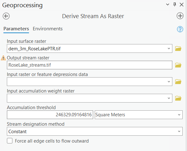
Identify the streams in your area of interest, either by using public data sets or deriving manually. In many cases, national-scale datasets offer a coarse representation of streams and it can be advantageous to derive them from high-resolution DEMs instead. Several methods exist for elevation-based stream derivation. We recommend the Derive Stream as Raster tool, which implements the Continuous Flow algorithm and does not require hydroconditioning.
Combine surface water bodies and streams
Combine the water bodies (reclassified DSWE) and streams rasters into a single, surface water raster using Raster Calculator. You can use the following expression format:
Con(~IsNull(<Reclassified DSWE>), <Reclassified DSWE>, <Streams Raster>)
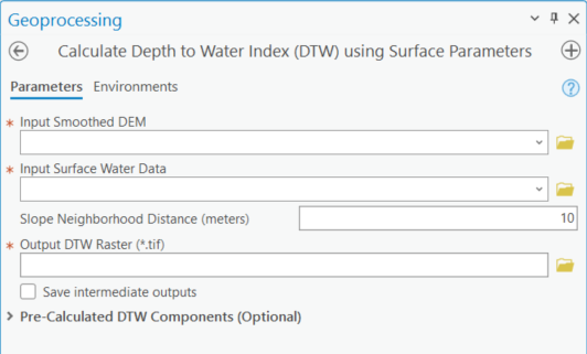
Derive Depth-to-Water Index
At this point, the created raster can be used directly as the Input Surface Water Data parameters for Calculate Depth to Water Index using Surface Parameters: