WIM User Guide
February, 2024
Download the WIM User Guide here
Executive Summary
The Wetland Identification Model (WIM) is an automated geoprocessing workflow created through research at the University of Virginia (O'Neil et al., 2018; 2019; 2020). The workflow predicts likely wetland areas from a set of hydrologically based indicators that are derived from a high-resolution DEM. WIM is implemented as a series of Arc Hydro Python Script Tools for ArcGIS Pro (version 2.5 and higher). This document describes the implementation of WIM within the Arc Hydro framework and its intended workflow.
Document History
Table 1. Document Revision History
| Version | Description | Date |
|---|---|---|
| 1 | Initial document (GLO). | March 2020 |
| 2 | Adding use cases and documenting step 0 | March 2021 |
| 3 | Updating use cases and documentation for Pro 3+ tools | February 2024 |
Getting Started with WIM
WIM is included in the installation of Arc Hydro Pro. Guidelines for installing Arc Hydro can be found here. Users should install version 2.0.165 or higher of Arc Hydro. Testing data used in this documentation can be found here.
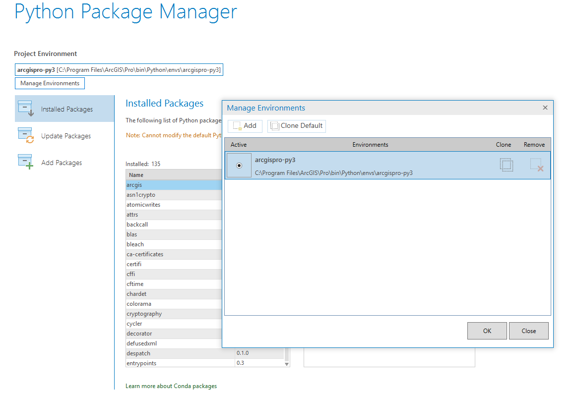
Users must also install the Scikit-Learn Python package to their ArcGIS Pro Python environment. Without doing so, "Train Random Trees," "Run Random Trees," and "Assess Accuracy" will fail. Follow the steps below to install the Scikit-Learn package.
Clone the default ArcGIS Pro Python environment.
In an ArcGIS Pro project, select the "Project" tab
Select the "Python" tab
Select "Manage Environments"
Select "Clone Default"
Add the Scikit-Learn package to the cloned environment.
With the cloned environment selected in the Python Package Manager page, select "Add Packages"
Navigate to Scikit-Learn and install the latest version.
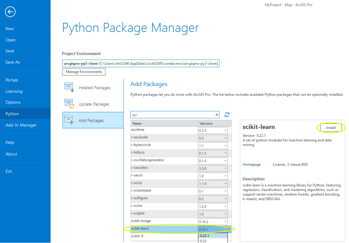
- Select the cloned environment as the activated Python environment before using the WIM tools.
Solution Overview
WIM is implemented as 10 script tools in the "Wetland Identification" toolset, within the Arc Hydro Tools Python Toolbox for ArcGIS Pro (Figure 1). The ModelBuilder implementation that was previously available has been removed as that execution method of WIM is not typically useful.
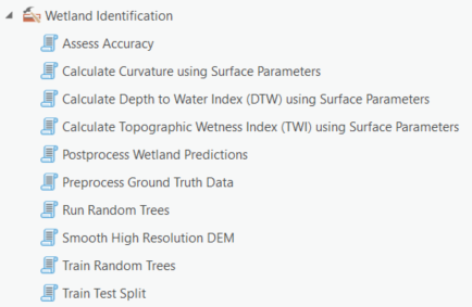
Figure 1. Arc Hydro Pro toolset implementation of the Wetland Identification Model
WIM consists of three main parts: preprocessing, predictor variable calculation, and classification and accuracy assessment (Figure 2). Required input data are a high-resolution digital elevation model (DEM), verified wetland/nonwetland coverage (i.e., ground truth data), and a surface water raster. Final model outputs are wetland predictions and an accuracy report. All workflow rasters must be in TIFF format. The intended workflow is:
(Optional) Input ground truth features are converted to raster format with the necessary environment settings applied.
The input DEM is smoothed to optimize the surface for hydro feature extraction.
The preprocessed DEM is used to calculate the predictor variables: the topographic wetness index (TWI), curvature, and cartographic depth-to-water index (DTW).
Training data are derived from the ground truth data.
The training data are coupled with the merged predictor variables to train a Random Trees (Breiman, 2001) model.
- Users can optionally incorporate other predictor variables in addition to or in place of the baseline topographic variables. The best-performing predictor variables may vary for different landscapes and target wetland types.
The trained Random Trees model is applied to an area to generate predictions.
The ground truth data that were not used to train the model are used to assess the accuracy of predictions.
(Optional) Apply simple, geometry based postprocessing to wetland predictions. This will also convert the raster prediction outputs to features.
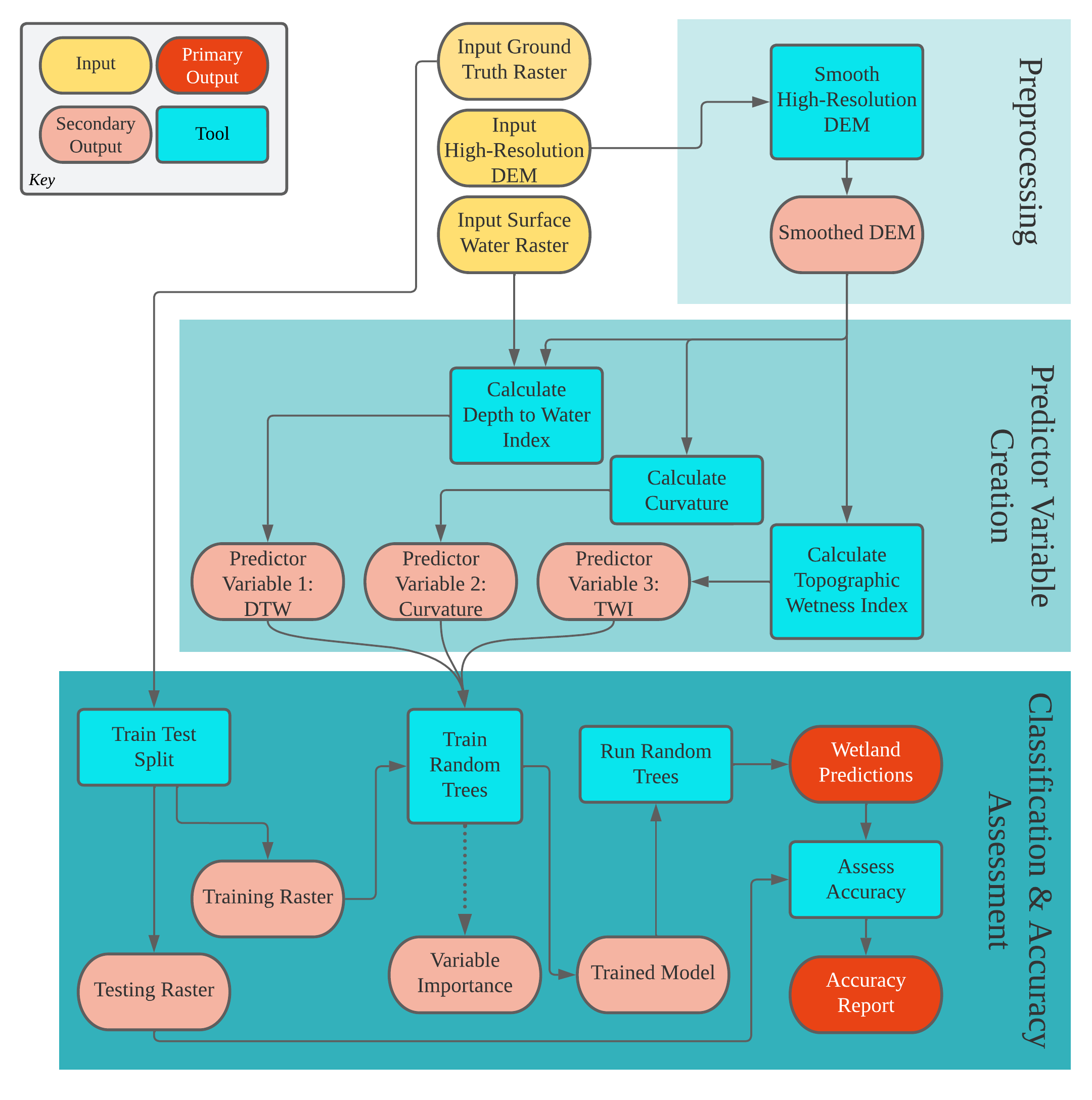
Figure 2. Overview of the Wetland Identification Model
Overview of WIM Tools
| Toolset | Step | Tool | Description |
|---|---|---|---|
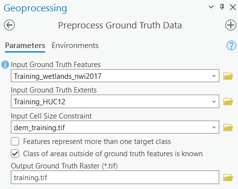
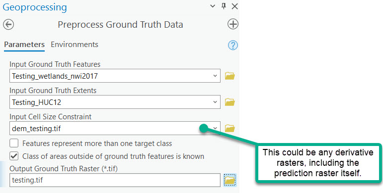
| Wetland Identification | (0 - optional) Rasterize ground truth features | Preprocess Ground Truth Data | Use this tool as a preliminary step to using WIM to ensure your ground truth raster input is in the proper format. Preprocess Ground Truth Data will return a raster with correct snap raster and cell size settings. The output raster will render known landcover classes (e.g., wetland or nonwetland) as integer raster values. Areas within the ground truth extents that are not known (i.e., unknown background areas) will be rendered as NoData and ignored in subsequent analyses. Users must take note of the integer value that represents specific classification targets. Integer values in the output raster must begin at 0 and increase by 1. The output raster will subsequently be used to create training and/or testing data. For that reason, the output raster dictates the cells that will be used for Random Trees training and accuracy assessments. |
(1) Smooth High-Resolution DEM | Smooth High-Resolution DEM | Smoothing is used to blur DEMs to remove the changes in elevation that are too small to indicate features of interest (i.e., microtopographic noise), which are ubiquitous in high-resolution DEMs. We recommend using a 3m resolution. | |
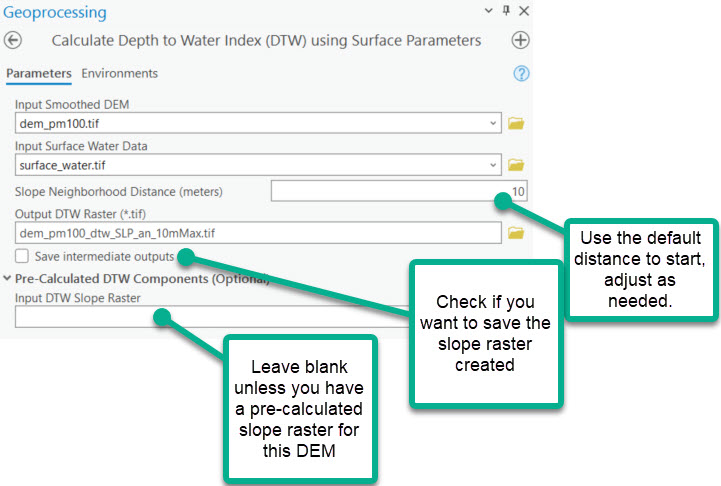
(2) Create Predictor Variables | Calculate Depth to Water Index | Calculates the cartographic depth-to-water index (DTW). The DTW, developed by Murphy et al. (2007), is a soil moisture index based on the assumption that soils closer to surface water in terms of distance and elevation are more likely to be saturated. This tool uses the Spatial Analyst Surface Parameters tool to calculate the slope component. Like Surface Parameters, this tool gives users the option to implement an adaptive neighborhood size to compute slope. Surface water inputs can be either raster or feature type. Users should derive DTW from a smoothed, high resolution DEM to avoid microtopographic noise, and should use updated surface water data. | |
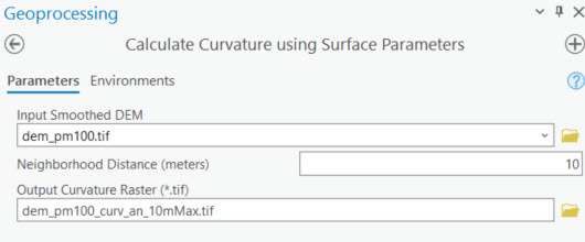
| Calculate Curvature | Calculates the curvature (i.e., the second derivative) of the land surface. Curvature can be used to describe the degree of convergence and acceleration of flow (Moore et al., 1991). This tool uses the Spatial Analyst Surface Parameters tool to calculate mean curvature. Like Surface Parameters, this tool gives users the option to implement an adaptive neighborhood size to compute curvature. Users should derive curvature from a smoothed, high resolution DEM to avoid microtopographic noise. | ||
| Calculate Topographic Wetness Index | Calculates the topographic wetness index (TWI). The TWI relates the tendency of an area to receive water to its tendency to drain water. This tool uses the Spatial Analyst Surface Parameters tool to calculate the slope component. Like Surface Parameters, this tool gives users the option to implement an adaptive neighborhood size to compute slope. To calculate the flow accumulation component, the tool uses the Spatial Analyst Fill tool or Spatial Analyst Derive Continuous Flow tool. Users should derive TWI from a smoothed, high-resolution DEM to avoid microtopographic noise. | ||
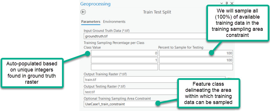
(3) Split ground truth data into a training set and a testing set | Train Test Split | Create training and testing subsets from a ground truth raster for supervised classification applications. The training raster is created by randomly sampling user-defined percentages of each discrete class of the ground truth data. Alternatively, the training raster is a subset designated by the training sampling area constraint. The testing raster is the complement of the training raster, comprised of all remaining cells in the ground truth extents. The testing raster represents a reserved group of ground truth cells that can be used to assess model accuracy for areas where it was not trained. | |
(4) Train the Random Trees model | Train Random Trees | Executes the training phase of the Random Trees algorithm. In this phase, the algorithm takes bootstrap samples of the training dataset. A decision tree is created from each bootstrap sample. Each decision tree attempts to learn patterns present in ground truth classes. The trained model is saved and can be used to generate predictions based on the patterns learned during training. | |
(5) Generate predictions | Run Random Trees | Predict the distribution of target landscape classes using a model trained for those classes. Predictions do not need to be made in the same area for which the model was trained, but the calculation of the predictor variable(s) used to train the model applied must be the same. In the baseline implementation, a model can be trained using the DTW, Curvature, and TWI for one area and used to make predictions for a new area where DTW, Curvature, and TWI have also been derived. | |
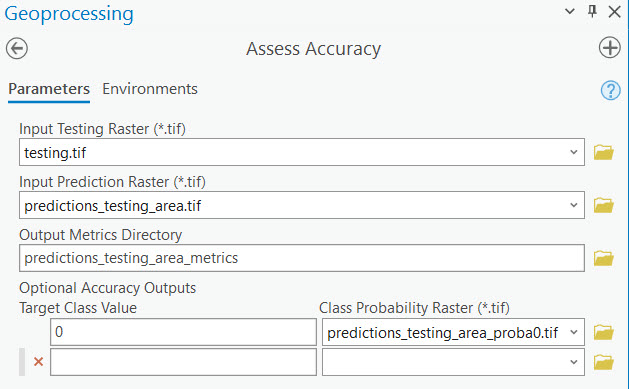
(6) Generate accuracy metrics for predictions | Assess Accuracy | Given the predicted output from the preceding step and a corresponding raster with ground truth labels for the cells (i.e., the testing raster), this tool generates accuracy metrics that summarize the model's ability to predict the target classes. Additional metrics are generated if the user includes output class probability rasters. | |
| (7 - optional) Apply geometry-based cleanup to wetland predictions | Postprocess Wetland Predictions | Pixel-based classifications, like Random Trees, can produce sparse predictions since they consider the relationship between target classes and characteristics on a cell-by-cell basis. In the case of wetlands, these isolated cells are unlikely to represent true wetlands, which exist as geomorphic objects. Further, smaller collections of sparse predictions may represent wetlands smaller than a user's minimum mapping wetland unit. This tool applies a simple, geometry based post-processing to raster wetland predictions to return a cleaned-up set of predicted wetland polygons. The post-processing workflow performs the following:
|
Database Design
It is recommended that you follow the intended database design. The folder structure is as follows.

Although the folder structure mirrors the Arc Hydro design, the Layers feature dataset is unused as no feature classes are created. The contents of the other folders are as follows.
"MyProject\Layers" subfolders:
"inputs"
Stores the input data in TIFF format. At a minimum, these data must include the DEM, ground truth dataset, and surface water raster. If a training area constraint is used, it should be saved to this location.
If running multiple trials of the WIM, the contents of this folder will not change.
"model"
Stores data that directly impact or are directly impacted by the Random Trees model. This includes the training and testing rasters, and the variable importance measures that are calculated each time a model is trained.
The contents of these files should be kept for reference over the course of trials that evaluate different training sampling scenarios.
"outputs"
- Stores the prediction outputs from the Random Trees model. This will always include a prediction raster, where each cell is assigned a class. This folder may also include prediction probability rasters.
"predictor_variables"
- Stores the predictor variables that are used to train the Random Trees model. If preprocessing parameters change, new contents will be added to this folder. If you choose to include additional predictor variables, they should be saved here.
"secondary_outputs"
- Stores intermediate raster outputs. These will include the smoothed DEM, hydroconditioned DEM, TWI components, and DTW components. If users have already used these rasters to derive predictor variables (see sections 2.3.3 - 2.3.5), the contents of this folder can be archived to free disk space.
"MyProject\train_model_predict_metrics" contents:
- This folder (named according to user input) contains the accuracy metrics used to summarize model performance. These are not GIS data, but rather various plots and tables.
Output Data Naming Conventions
It is best practice to follow predetermined data and naming conventions. These include the following:
Processed DEMs are saved with prefixes that describe the preprocessing methods applied. For example, "dem_pm_100.tif" is a DEM that was smoothed using the Perona-Malik method with 100 iterations.
By default, predictor variables are saved with the base name of the preprocessed DEM and a suffix with the pattern "_[var].tif." This is recommended to keep track of the effect of DEM preprocessing on wetland modeling accuracy, and how the best-performing preprocessing methods may differ across predictor variables.
Training and testing rasters are saved as "train.tif" and "test.tif" by default. However, users are encouraged to choose names that reflect the training sampling scenario applied, since the base name of the training raster is used for naming prediction and accuracy outputs. An example of recommended naming convention would be "train_0_50_1_20.tif" and "test_0_50_1_80.tif". These names reflect that 50% of class 0 and 20% of class 1 were used for training, and the accuracy assessment will apply to the remaining 50% and 80% of class 0 and 1, respectively.
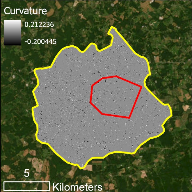
Extents and Size Limitations
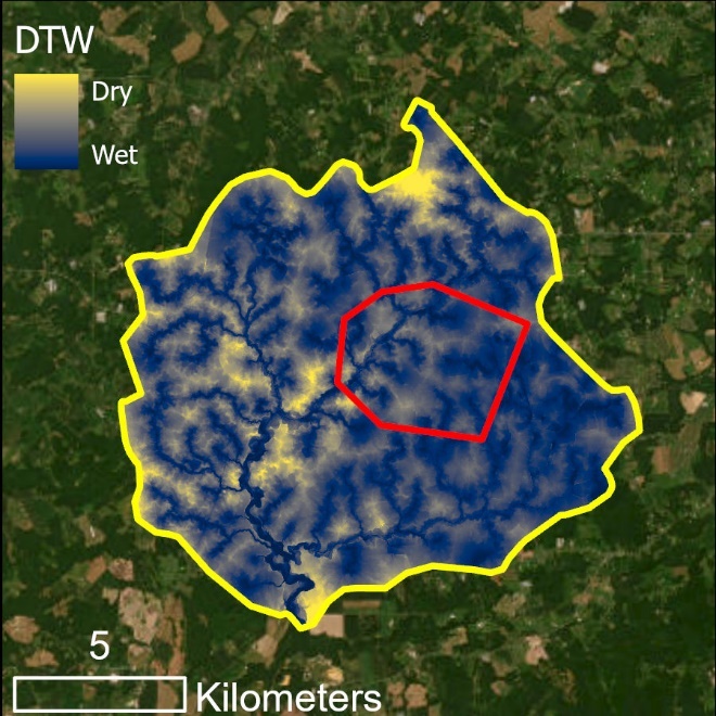
There are two distinct processing extents when running WIM (Figure 3). First, is the modeling extent. The modeling extent is determined by the ground truth area extents. This represents the area for which a model can be trained and tested because the true landcover classes are only known within these extents. The Train Random Trees tool will only process within the extents of the training raster. The Assess Accuracy tool will similarly only process within the extents of the testing raster.
Second is the predictor variable extent. This extent represents the area for which wetland characteristics are generated. The best practice for this extent is the smallest hydrologic unit that encompasses the modeling extent, as this will allow the user to include the area's hydrologic connectivity. Due to raster size limitations, the predictor variable extent should not be larger than a HUC-12 watershed with 1m resolution, and smaller watersheds are encouraged if available. Using the baseline implementation of WIM, the predictor variable extent is determined by the input DEM and surface water raster. If users include additional predictor variables, such as imagery-based vegetation information, the source imagery raster would also determine the predictor variable extents. The predictor variable extent is the processing extent used for all tools other than Train Random Trees and Assess Accuracy. Moreover, wetland predictions can be generated for the entirety of the predictor variable extent, as seen in the use cases.
Size limitations for input rasters will vary by machine. On the backend, raster size limitations are determined by NumPy array size limits and limits inherent to the arcpy RasterToNumPyArray tool. If users run into size-related errors, they should process in chunks. For example, derive the predictor variables in watershed chunks (no larger than a HUC-12) and use the most confident pocket of ground truth data to train the model, reserving other areas for accuracy assessment. We recommend following the WIM workflow with a 3m raster resolution, stemming from a 3m DEM resolution. In most cases, this resolution allows for processing of an entire HUC-12. In addition, wetland modeling has been shown to achieve a higher accuracy when predictor variables are modeled from a 3m DEM vs. 1m.
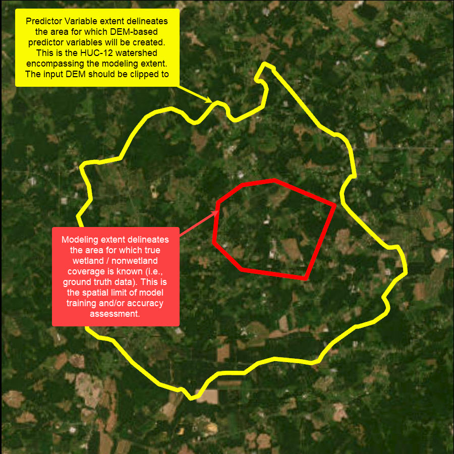
Figure 3. WIM modeling extent (red) and predictor variable extent (yellow). The predictor variable extent is a hydrologic unit that fully encompasses the ground truth area. The modeling extent (red) is the ground truth area, where training and testing can occur. If ground truth data extends to an entire watershed, the predictor variable and modeling extent would be the same (as shown in Use Case 1).
Use Cases
WIM is intended to produce an initial screening of wetlands in areas where wetlands data does not exist. WIM outputs can be useful for understanding relative wetland abundance between areas and/or prioritizing surveying efforts to manually confirm wetland characteristics.
WIM is flexible and can be configured to fit several modeling needs. Below, we provide suggestions and starting points for WIM parameters. But users should keep in mind that optimal WIM parameters will vary by the landscape and application. It will be an iterative process to build the best-performing model for a user's specific study area and end goal. For more detailed discussion on the methods applied and the justification for their use in the WIM workflow, see O'Neil et al. (2018; 2019).
The following use cases are chosen to highlight the flexibility of WIM. Use cases are based in Delaware and leverage updated NWI data as ground truth data. However, we recommend using the most accurate ground truth data available for your own applications.
Follow along with Use Case data. This data package will include all input and created data, with the exception of trained model files.
Use Case 1 - Binary Classes, Baseline Predictor Variables, Training Sampling Constraint
Use Case 1 applies WIM with binary ground truth classes (e.g., wetlands and nonwetlands) and only the baseline predictor variables (i.e., curvature, TWI, and DTW). All ground truth data is contained by a single HUC-12 watershed, so we will use a training sampling area constraint to create distinct training and testing datasets.
Our input data for this use case is as follows:
Ground truth wetland features,
One feature delineating the extent to which wetlands were surveyed (i.e., all areas within the extents other than wetlands are confidently nonwetland area),
One feature delineating the extent within which training data can be extracted,
DEM raster (3m resolution), and
Surface water raster.
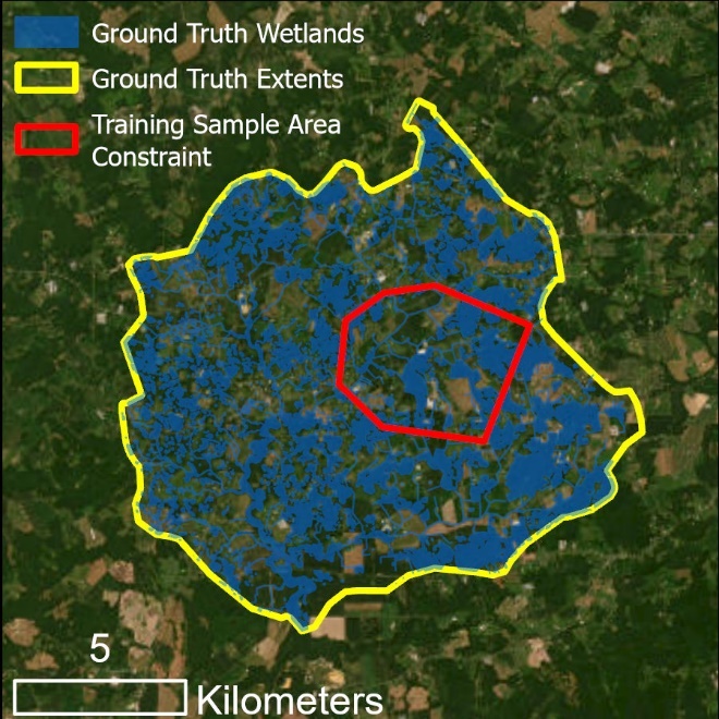
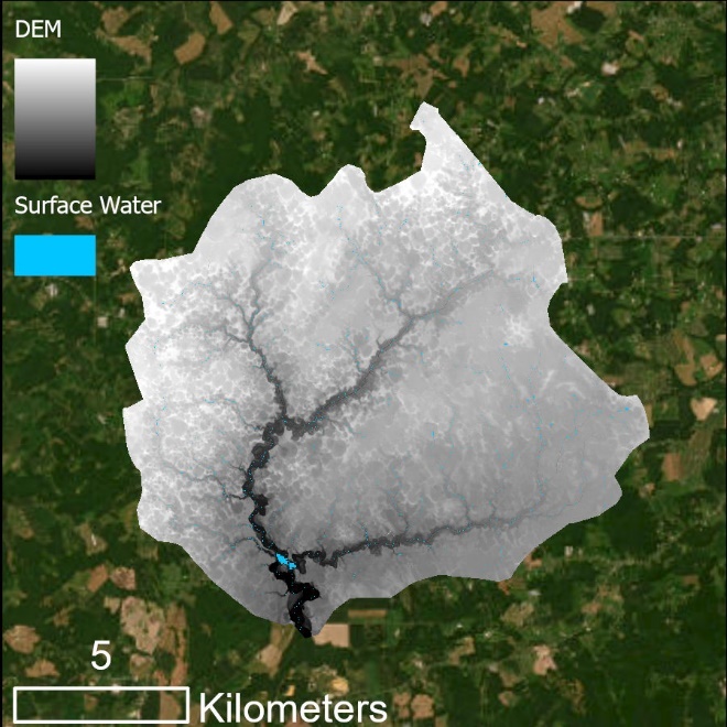
Input data for Use Case 1, separated by feature data (left) and raster data (right)
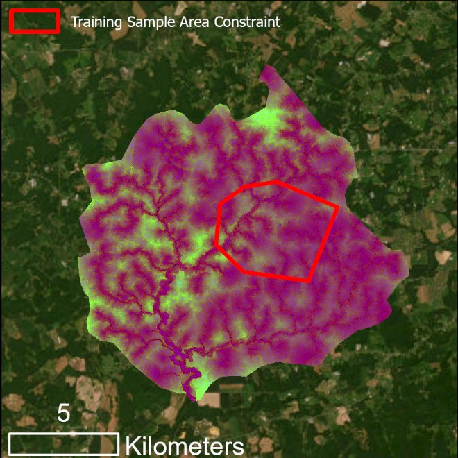
Note that in this example, wetland coverage is known within an entire HUC-12 watershed. Unlike the example in Figure 3, the predictor variable extent and the modeling extent are the same - the HUC-12 boundary (yellow). The DEM was clipped to the HUC-12 extent and predictor variables will be calculated for that area. The model will train using data within the training sampling area constraint (red), which delimits the training data. Model predictions and accuracy assessment will be completed for the area outside of the training sample constraint and within the HUC-12 boundary, i.e., the extent of the testing data. See the visual illustrations below.
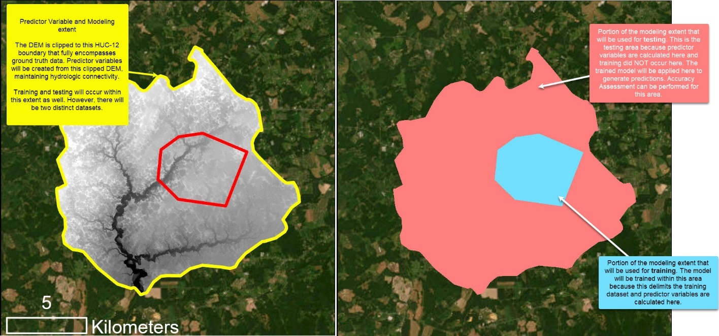
Explanation of the computational extents for Use Case 1
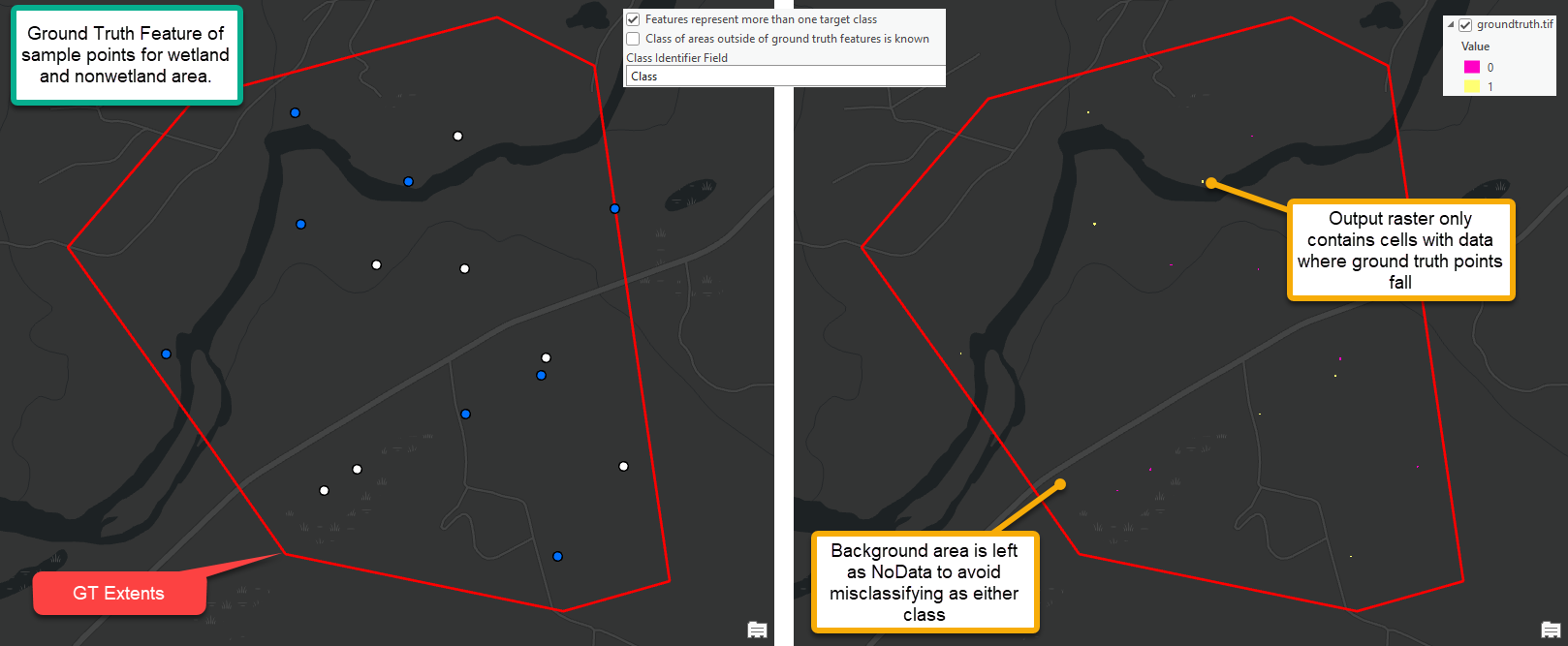
0. Preprocess Ground Truth Data
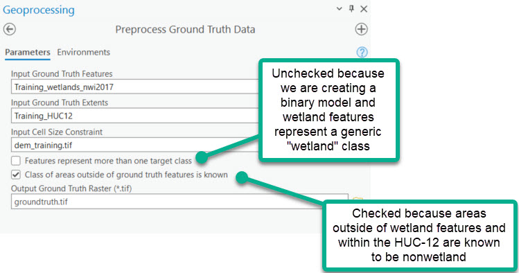
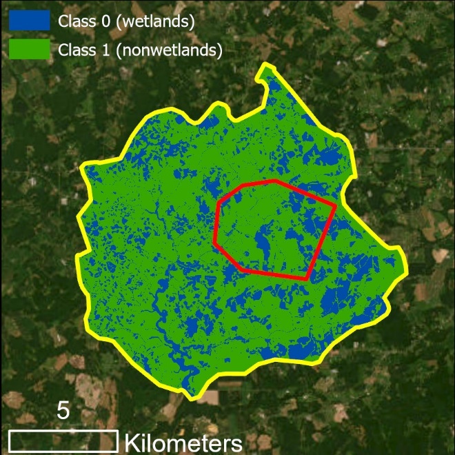
Ground truth raster output created by Preprocess Ground Truth Data
The Preprocess Ground Truth Data tool converts ground truth features and the limits of known ground truth area into a raster with resolution, spatial reference, and extent that matches the input DEM. The created ground truth raster represents known landcover classes as unique integer values. In the example above, pixels with a value of 0 correspond to known wetlands and those with a value of 1 correspond to known nonwetlands. These pixels will be interpreted by the Random Trees model as target classes. See following sections for details on configuring a model with multiple target classes.
1. Smooth High Resolution DEM
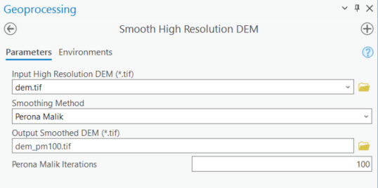
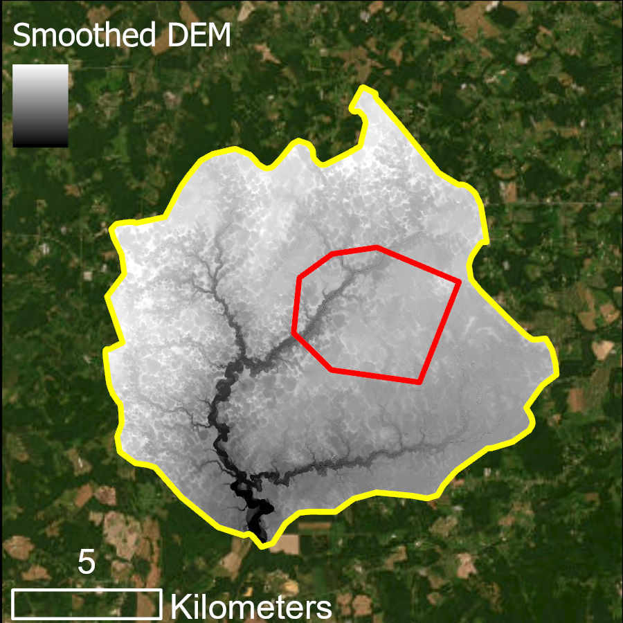
Smoothed DEM created by Perona Malik Smoothing via Smooth High-Resolution DEM
We strongly recommend the Perona Malik Smoothing algorithm for hydrologic feature extraction. Applying this smoothing process has been shown to improve both stream extraction (Passalacqua et al., 2010) and wetland (O'Neil et al., 2019) modeling.
2. Calculate Predictor Variables
In this step, rasters that describe wetland and nonwetland characteristics are prepared. We focus on the three baseline WIM predictor variables. These are topographic derivatives that serve as proxies for near-surface soil moisture. Other wetland/nonwetland indicators can be included, and in some cases, should be included to improve models.
1. Calculate Depth to Water Index (DTW)
The DTW calculation requires an input surface water raster. These data may come from public datasets for streams and waterbodies, such as NHD. Or they may be derived from a combination of satellite imagery and the elevation data. See this blog on creating a surface water raster for WIM using DSWE and elevation-derived streams. In any case, the surface water raster must have the same resolution and projection as the input DEM.
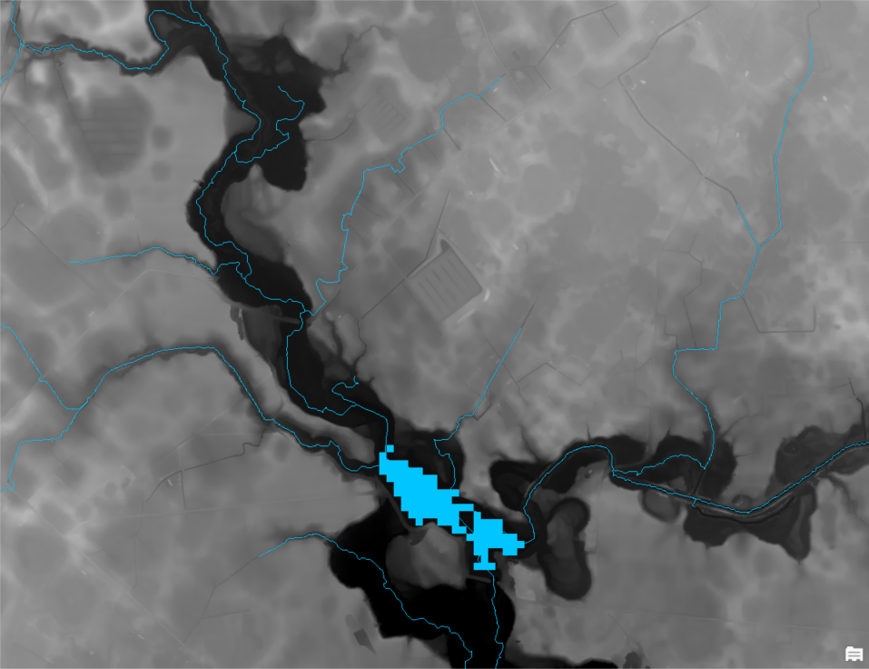
Example of the input surface water raster showing stream centerlines and waterbody as observed by DSWE.
DTW results for the predictor variable extents (left) and zoomed in showing known wetlands in white shading (right).
2. Calculate Curvature
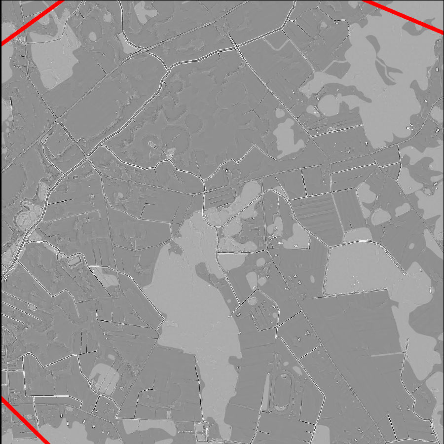
Curvature results for the predictor variable extents (left) and zoomed in showing known wetlands in white shading (right).
3. Calculate Topographic Wetness Index (TWI)
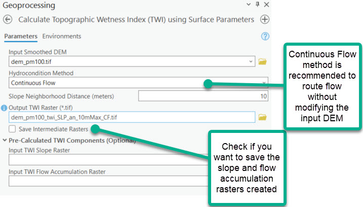
We recommend using the Continuous Flow option for the Hydrocondition Method. This method leverages the A* least-cost path analysis for flow routing, where water is routed into sinks along the steepest path and out of sinks along the mildest ascent. This method allows us to omit altering the high-resolution DEM through Fill or similar hydroconditioning techniques.
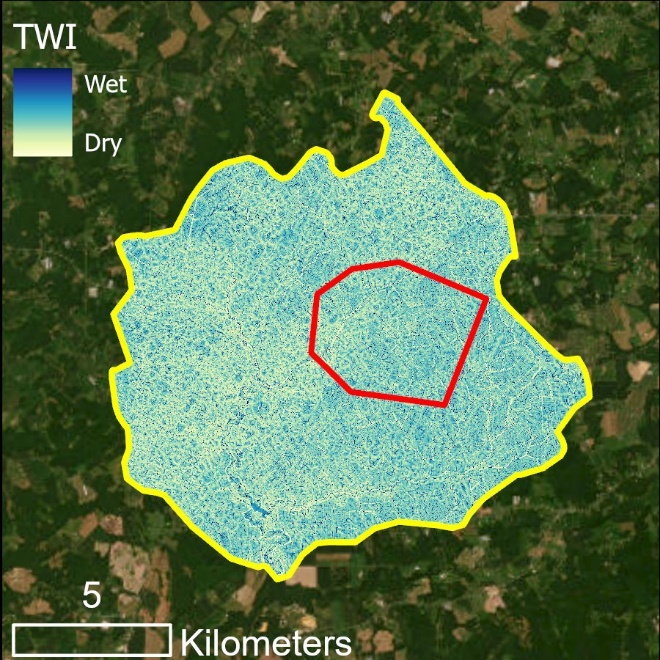
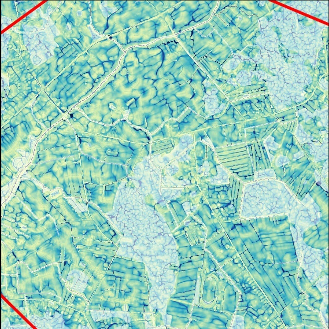
TWI results for the predictor variable extents (left) and zoomed in showing known wetlands in white shading (right).
3. Train Test Split
Train Test Split is used to partition the prepared ground truth data into training and testing subsets. The training subset represents the only areas of ground truth data seen by the model to learn the relationships and dependencies between the predictor variables and the ground truth classes. The testing subset is reserved ground truth data that can be used to assess how accurate predictions are for an area where the model was not trained. An alternative to this application of Train Test Split is the one shown in Use Case 2.
Aside from the methods shown here and in Use Case 2, users could alternatively skip this step and proceed to training the random trees model with the entire ground truth raster. However, the ground truth area would then be disqualified for a representative accuracy assessment.
Note that without a training sampling area constraint, you may want to modify the Percent to Sample for Testing parameter. For example, if training data can be sampled from the entire ground truth area, a user could specify that only 50% from each target class should be sampled for training and the remainder would be left for testing. The Percent to Sample for Testing can also be used to address class imbalance. In an area with significantly more wetland area than nonwetland, it can be beneficial to sample a smaller proportion of the nonwetland class to provide more similar quantities of wetland and nonwetland examples during training.
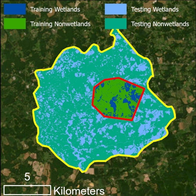
Training and testing rasters created by Train Test Split
4. Train Random Trees
In this step, a Random Trees model is created that defines dependencies between the predictor variables and wetland vs. nonwetland presence. You may encounter a warning that rasters will be clipped to maintain common extents. That is expected and not a cause for concern.
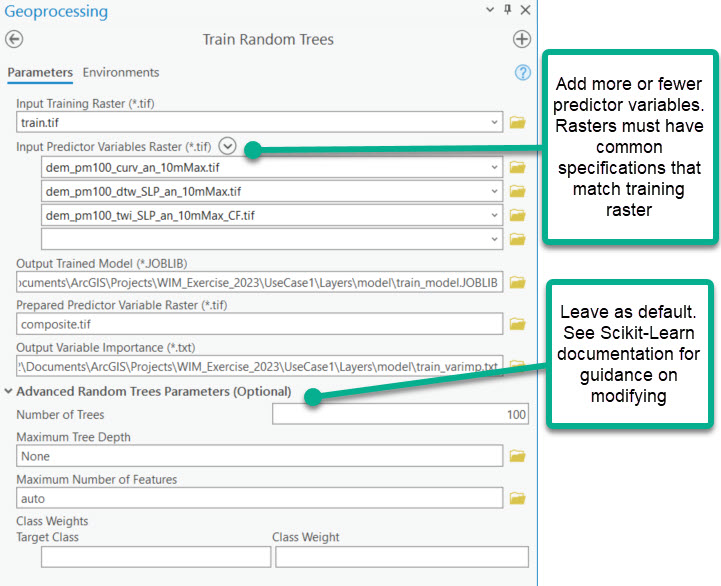
This tool creates several important outputs:
Composite raster
- Multidimensional raster where each band stores the information from one of the predictor variables. If only one predictor variable is used, the composite raster will be a copy of the single predictor variable. If you already have a composite raster of your predictor variables, you can enter that as the single predictor variable raster.
Variable importance report
- Relative measures of importance between the predictive variables during training. The values are related to an estimated decrease in accuracy if that variable were removed.
Trained model (*.JOBLIB)
- File that retains the learned relationships between predictor variables and target classes. This file can be used to generate new predictions.
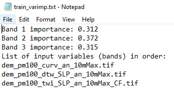
Outputs from Train Random Trees, variable importance report (left) and composite raster (right)
The composite raster is created from the three predictor variable rasters; thus, it maintains the full predictor variable extent. However, the model training only occurred within the extents of the training dataset (red extents).
5. Run Random Trees
The resulting trained model can now be applied to any composite raster comprised of the same combination of predictor variables, in the same order. We will generate predictions for all of the composite raster. The output predictive rasters will contain results for an area that the model has already learned from as well as a larger area where the model has not been trained.
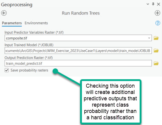
Two sets of outputs are created:
One prediction raster that represents the hard classification. Each pixel in this raster is assigned the class that the model predicts it belongs to.
Probability raster created for each target class from training. Each pixel in the rasters is assigned a probability (0-1) that it belongs to the corresponding class.
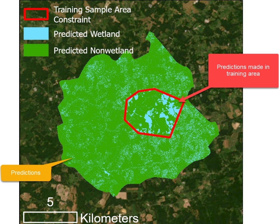
Output predictions for Use Case 1, where each pixel is assigned a predicted class.
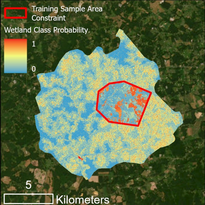
*Output class 0 (i.e., wetlands) probability predictions for Use Case 1, where each pixel is assigned its probability of belonging to class 0.*
6. Assess Accuracy
Predictions were generated in areas outside of the training area, i.e., the testing area. Since we know the true coverage of wetlands and nonwetlands within the testing area, we can perform an accuracy assessment and understand the trained model's expected accuracy in similar areas. The Assess Accuracy tool will compare the predictive value of each pixel to the actual pixel value, according to the testing raster.
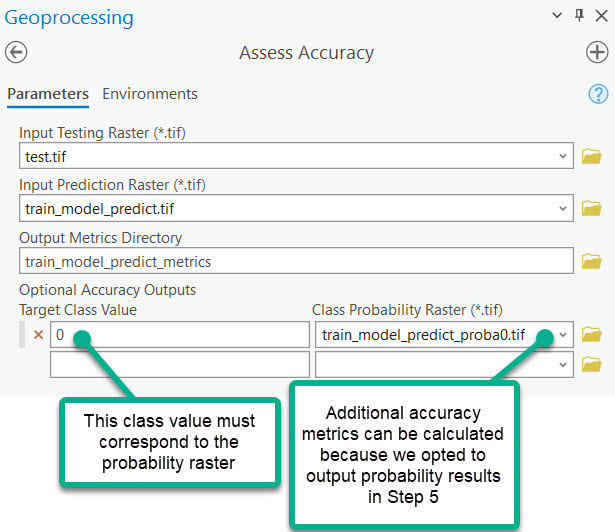
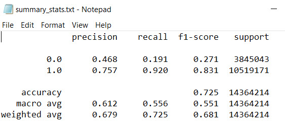
A directory of accuracy metrics is created. The accuracy metrics pertain only to the extents of the testing raster used in Assess Accuracy. The Scikit-Learn library is the engine behind the accuracy metrics. The accuracy results include:
- Accuracy report - summarizes the precision, recall, and F1-score of each prediction target. The "support" column is the number of pixels per class in the testing dataset.
- Confusion
matrix
- summarizes the number of pixels in the prediction raster that falls into the true positive, true negative, false positive, false negative categories.
- Precision-Recall
curve
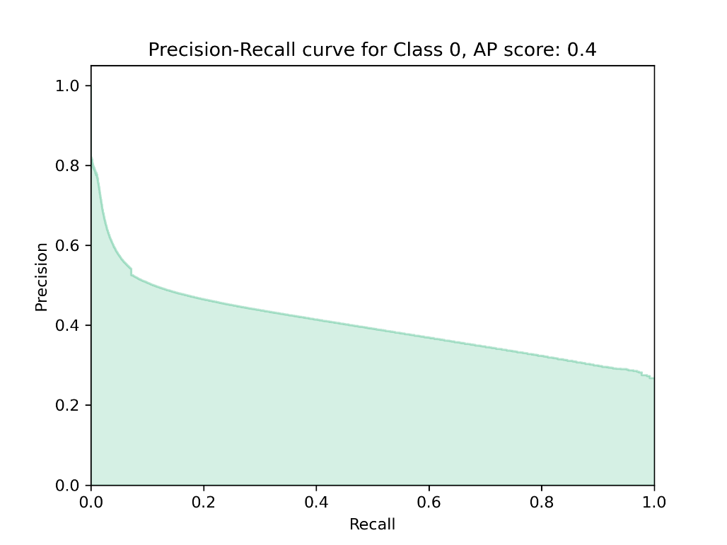
- plots the precision and recall for varying decision thresholds, as given by the probability raster. This output is only created if Optional Accuracy Outputs are entered. The precision-recall curve also gives an Average Precision score, which summarizes the accuracies overall. A perfect mode will have an Average Precision of 1. Strong models are those that trend towards Average Precision = 1.
Interpreting Use Case 1 Results
While the WIM workflow was executed successfully for Use Case 1, the model performed poorly. Average Precision was relatively low (0.4), and wetland precision and recall were low (47% and 19%, respectively).
This specific study area is agricultural, which may impact natural drainage patterns and result in misleading wetland signatures from the baseline wetland indicators alone. For that reason, our model may benefit from being able to relate wetlands to landcover classes, in addition to topographic indices. In Use Case 2, we will refine the model by adding landcover data to the predictor variable set.
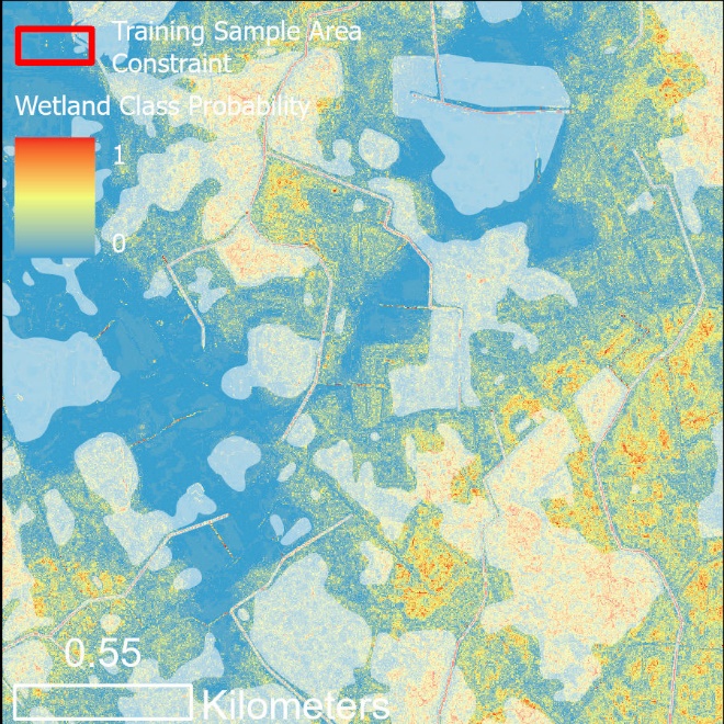
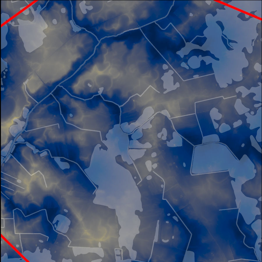
Use Case 1 Probability results with known wetlands shown (white shading). This scene exemplifies the poor performance of the Use Case 1 model, where known wetlands are predicted to have low-medium wetland likelihood.
Use Case 2 - Additional Predictor Variables
WIM baseline indicators may be insufficient for wetland modeling in areas with built drainage or landscapes with a more complex subsurface (e.g., coastal or glacial influence). In such cases, topographic variations do not correlate well to ground water table gradients, which is an underlying assumption of WIM's baseline inputs. Even in areas where the baseline topographic derivatives are good indicators of wetlands, additional predictor variables may improve results by providing more distinct characteristics for target classes.
WIM predictor variables are not limited to DEM-derived indices. The Random Forests algorithm can train on both continuous and categorical data. So, WIM inputs can include other indices, like NDVI, as well as discreet and non-ordinal data like landcover classes.
This specific study area is agricultural, which may impact natural drainage patterns and result in misleading wetland signatures from the baseline wetland indicators alone. For that reason, landcover class information may improve our model by indicating cropland vs. natural areas.
We will refine the Use Case 1 model by adding landcover data from the Living Atlas. Refer to Use Case 1 for steps 1 - 3.
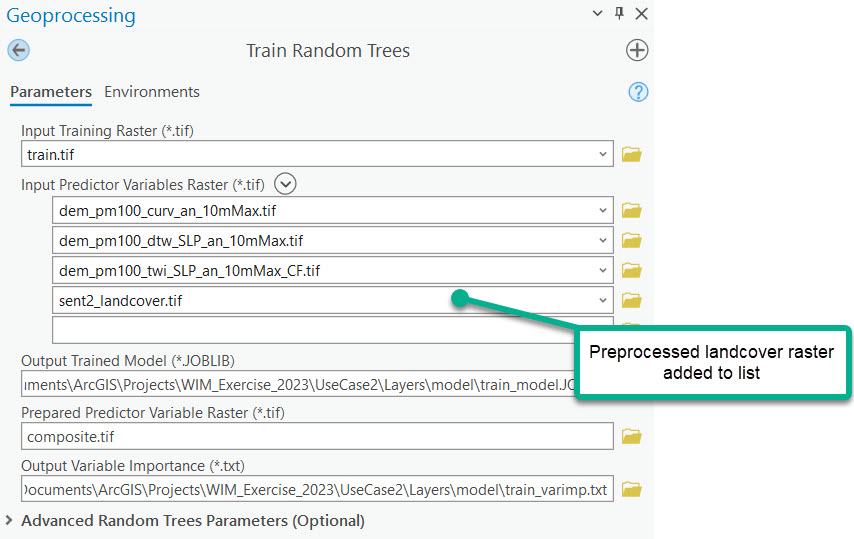
4. Train Random Trees - Additional Predictor Variable
4a) Preparing additional predictor variables
As with any additional predictor variable, this dataset must be exported as a TIFF with matching cell size, projection, and extents as the input DEM. This can be accomplished with several tools. We used the following procedure:
Run Extract By Mask
Input raster = raw landcover raster
Input raster mask data = preprocessed DEM (has been clipped to the processing extents and is in the desired projection)
Extraction Area = inside
Environments
Output Coordinate System = preprocessed DEM
Processing Extent = preprocessed DEM
Cell Size = preprocessed DEM
Snap Raster = preprocessed DEM
4b) Train Random Trees
The newly generated variable importance report provides a sense of the value provided by the additional predictor variable.
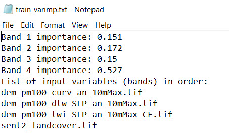
Variable Importance report generated from Train Random Trees with the additional predictor variable, landcover classes
The landcover class input appears to be impactful as it has a higher importance than the three baseline inputs.
5. Run Random Trees
Just as we did in Use Case 1, Run Random Trees will be used to generate predictions with the newly trained model. This iteration of the tool will use the model file and composite raster created in the previous step. The newly trained model can only be applied to composite rasters composed of the same four predictor variables: curvature, DTW, TWI, and Sentinel 2 landcover classes.
We can see the effect of our model refinement by comparing these results to Use Case 1 results.
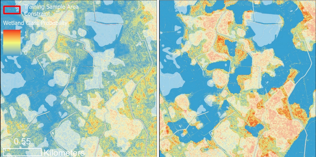
Wetland class probabilities predicted by the Use Case 1 (left) and Use Case 2 (right) models. Use Case 1 leverages only the baseline WIM predictor variables. Use Case 2 adds Sentinel-2 landcover classes to the predictor variable set. Verified wetlands are shown in white shading.
A visual comparison between the Use Case 1 and Use Case 2 results show the Use Case 2 model was more certain in wetland predictions within the testing wetlands. This indicates a more accurate model.
6. Assess Accuracy
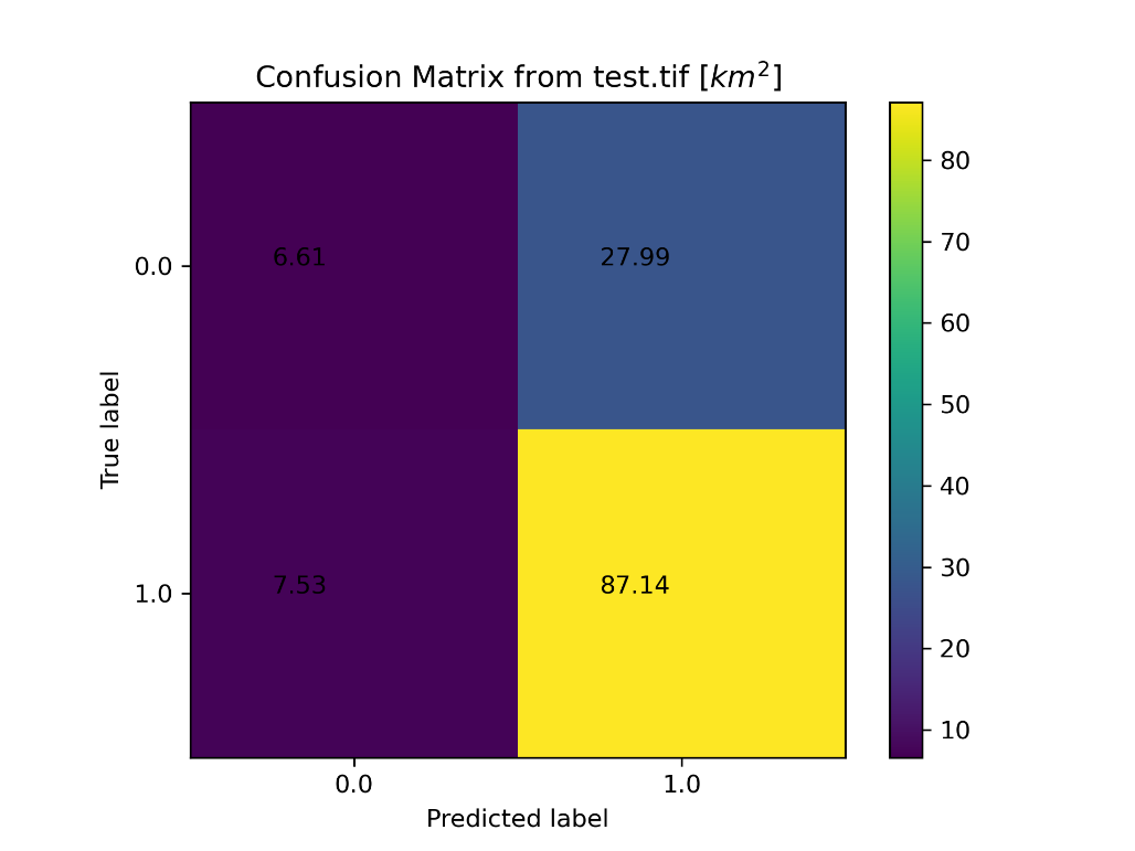
Following the method in Use Case 1, an accuracy report can be generated for Use Case 2. The same testing dataset is used, but they are compared to the Use Case 2 results. Shown below, the inclusion of landcover data improved the model according to all accuracy metrics.
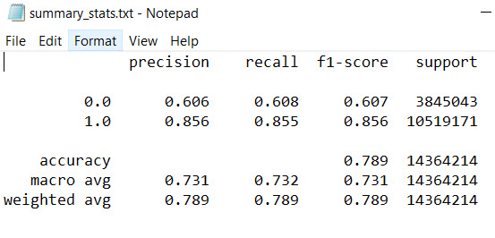
Accuracy report for the Use Case 2 model
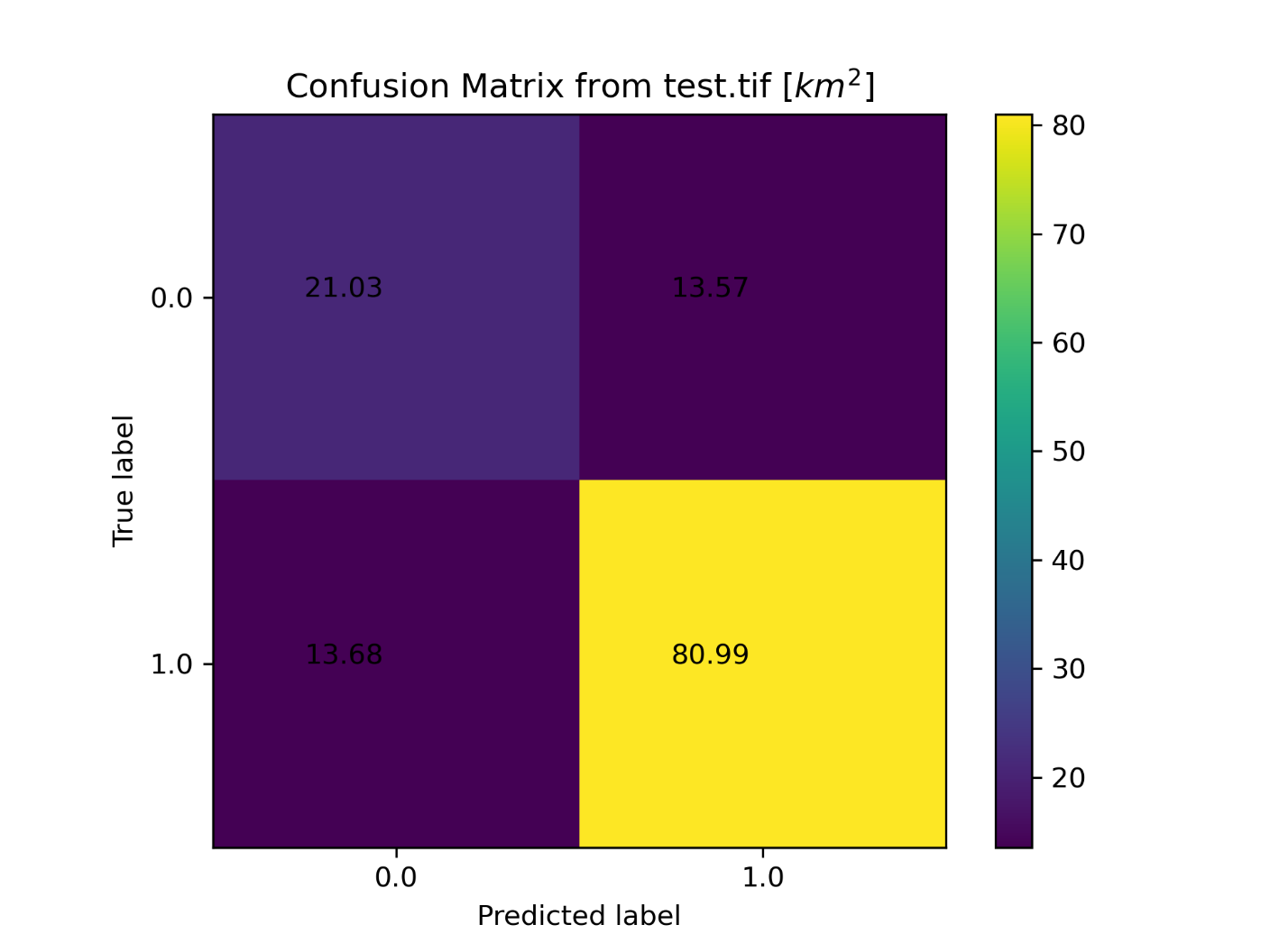
Confusion matrix for the Use Case 2 model
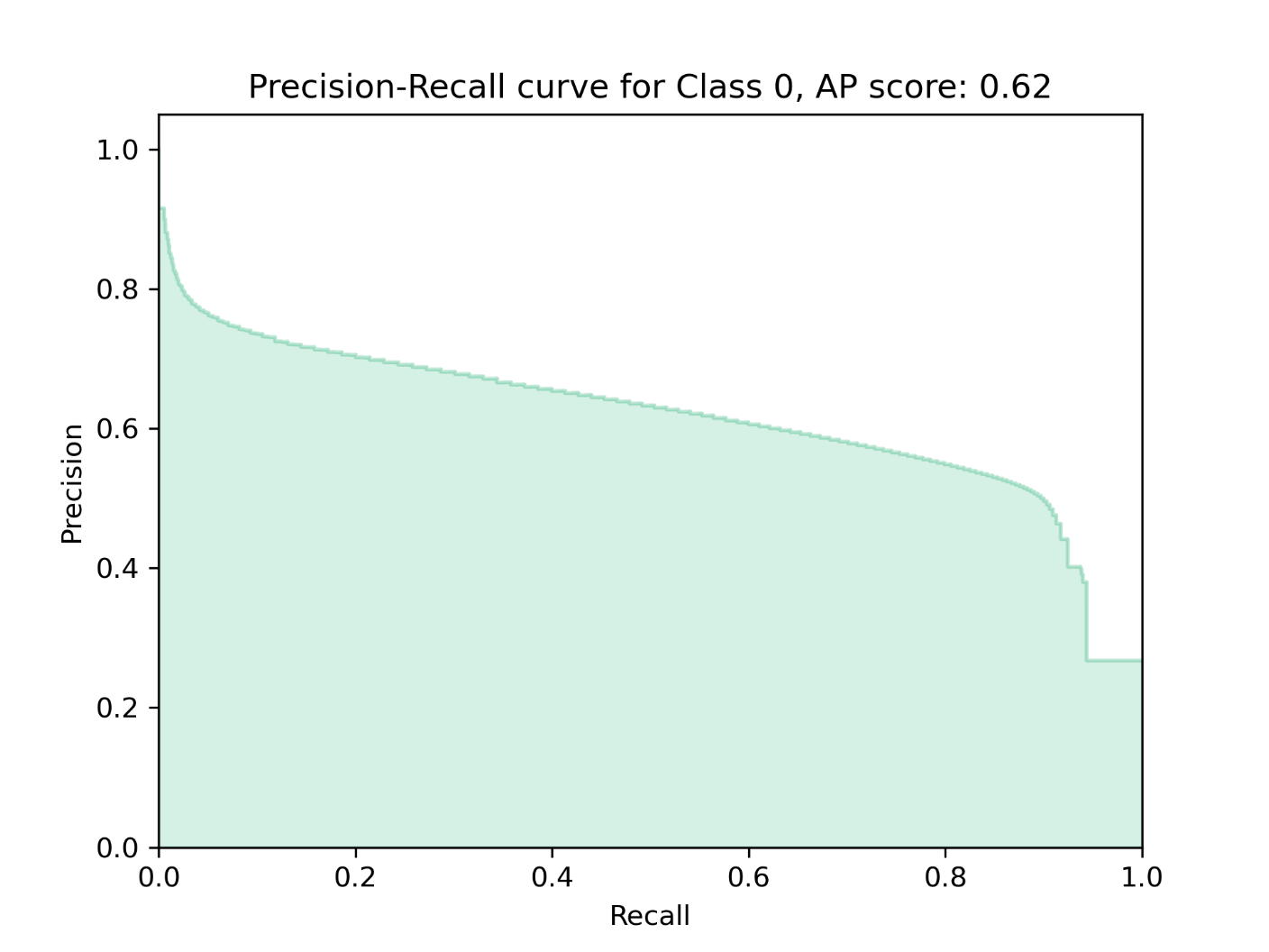
Precision-recall curve for the Use Case 2 model
Use Case 3 - Applying a Developed Model to a Similar Area
Use Case 1 and Use Case 2 describe a scenario where a user has a single HUC-12 area of interest, and a portion of that area is used to train a model while the remainder is used to run inference and assess accuracy. Another typical scenario is one where a model is developed in one region for which wetland distribution is known (perhaps one HUC-12) and applied to a new region where wetlands data does not exist. In this scenario, the separate training and testing regions should have similar enough landscapes that the learned wetland characteristics are likely to translate. As with the previous examples, the model must be applied to an area that has the same predictor variable set that was used for training.
Use Case 3 entails training a model using one HUC-12 and testing and evaluating the model in an adjacent HUC-12. Data from previous use cases are repurposed.
Our input data mirrors the Use Case 1 set; however, data is available for two HUC-12s (training and testing HUC-12s). Since ground truth data is known for all of the Training HUC, the entire Training HUC is the predictor variable extent. Training will occur for all pixels within the Training HUC. We will calculate predictor variables for all of the Testing HUC, so the trained model will be applied for the entirety of that area. Testing wetlands are known for all of the Testing HUC, so an accuracy assessment will be performed for the entirety of that area as well.
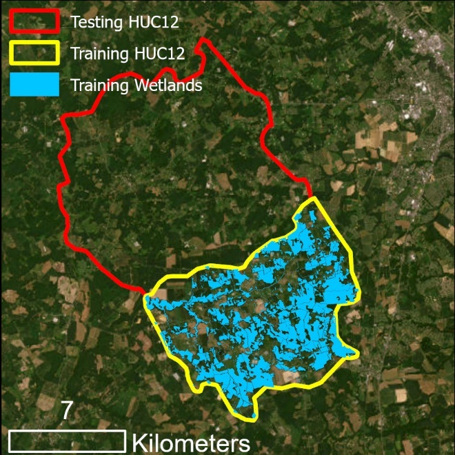
Training (yellow) and testing (red) areas for Use Case 3. All wetlands in the training area will be used to train a model that will be applied to the testing area.
0. Preprocess Ground Truth Data
Run the Preprocess Ground Truth Data tool for the training dataset. Save the output as training.tif.
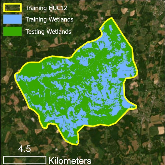
Training raster for Use Case 3
1. Smooth High-Resolution DEM
Repeat Step 1 from Use Case 1 using the DEM for the training HUC12. This will create a Perona-Malik smoother DEM in the training area.
2. Calculate Predictor Variables
Repeat Steps 2a, 2b, and 2c from Use Case 1 using the DEM for the training HUC12. These steps will create the following:
Curvature for the training area
TWI for the training area
DTW for the training area
In addition, we will again use a landcover raster derived from Sentinel-2, as we did in Use Case 2. A prepared landcover raster is provided for you in the UseCase3 > Layers > predictor_variables directory.
3. Train Test Split
We will use the entirety of the ground truth raster in the training area (i.e., "training.tif") to train the model. This raster was created with the necessary environment constraints during the Preprocess Ground Truth Data tool. For that reason, Train Test Split is skipped.
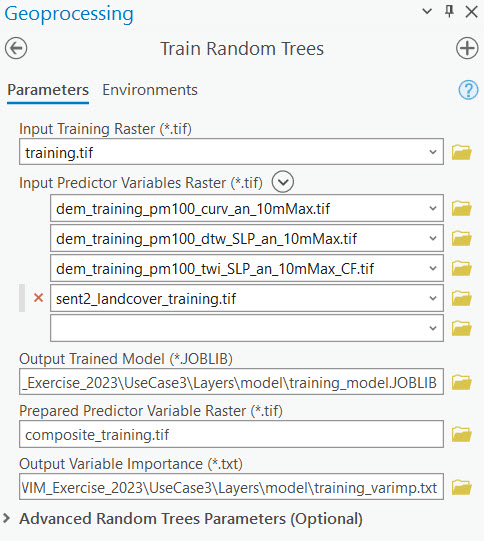
4. Train Random Trees
Use the Train Random Trees tool to train a model within the training extents. Save the Prepared Predictor Variable raster as composite_training.tif. As done in previous use cases, leave all advanced parameters as the default values.
5. Run Random Trees
Before generating predictions in the testing area, we must create a composite raster for the testing area that mirrors the predictor variable set used to train the model in Step 4.
i. Smooth High-Resolution DEM
Smooth the testing DEM using the same parameters applied to the training DEM in Step 1.
ii. Calculate Predictor Variables
Create Curvature, TWI, and DTW rasters from the smoothed testing DEM. Use the prepared surface water raster for the testing area that is provided.
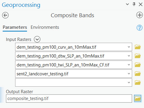
iii. Create a composite raster
Use the Composite Bands tool to create a composite raster for the testing area. Be sure to enter the rasters in the same order as was used in Step 4.
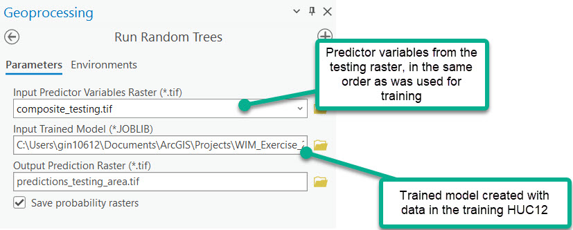
iv. Generate predictions with the trained model
Use the Run Random Trees tool to generate predictions for the testing area.
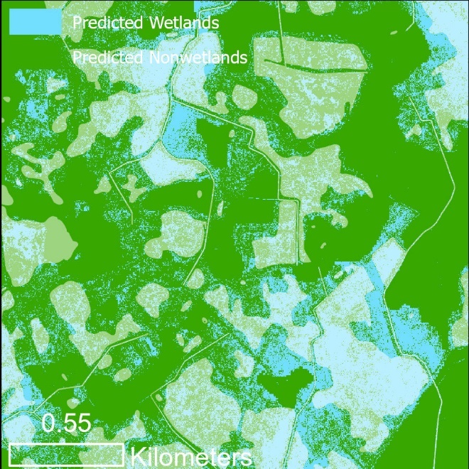
Prediction results for Use Case 3, verified wetlands are shown in white shading.
6. Assess Accuracy
Predictions have been generated within the testing HUC12. We have verified wetlands for this same area; thus we can perform an accuracy assessment.
i. Use Preprocess Ground Truth Data to prepare the testing wetlands data for Assess Accuracy
ii. Assess Accuracy
Use the output from the previous step (testing.tif) as the testing raster input to assess the accuracy of the prediction results.
Additional Usage Guidance
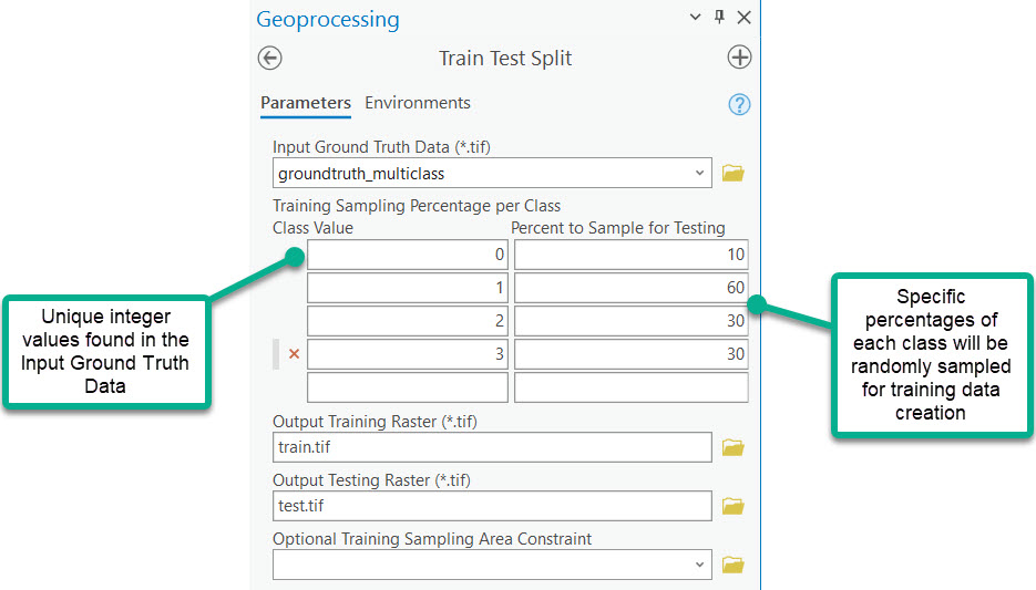
Multiple Target Classes & Specific Sampling Percentages
Seeing an example below for using WIM with multiclass ground truth classes (e.g., wetlands by type or wetlands and specific nonwetland classes). Additionally, specific sampling percentages will be indicated for training data sampling.
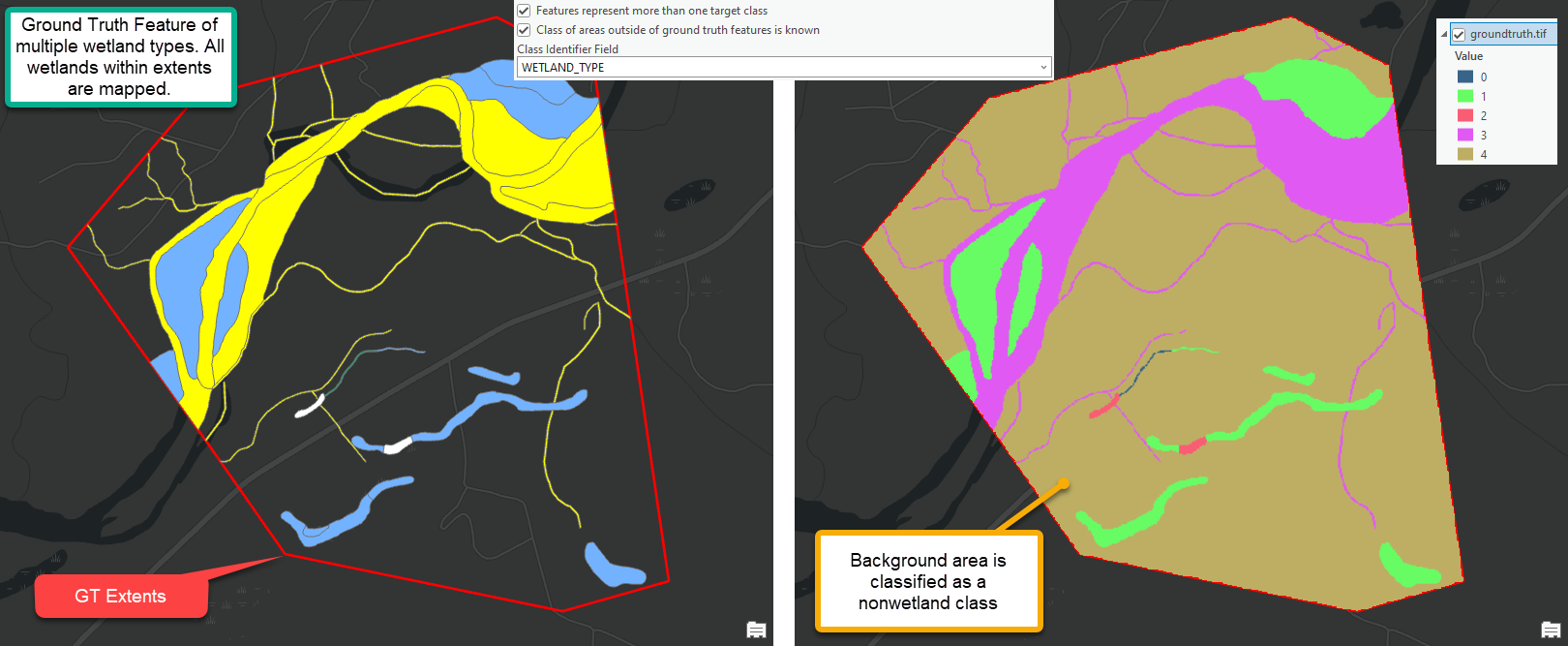
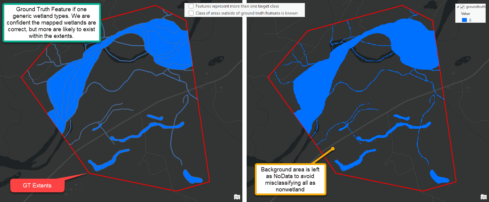
Assume the Input Ground Truth Features are polygons that represent multiple known landcover classes. The distinct classes are indicated by the "type" field. Preprocess Ground Truth Data can be used to rasterize these features properly for WIM, while maintaining the class data.
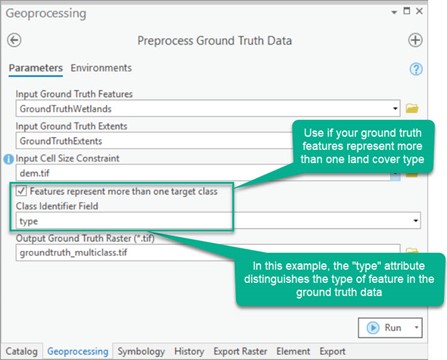
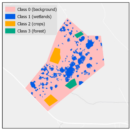
Groundtruth raster created with multiple classes
See additional examples for Preprocess Ground Truth Data here.
The Train Test Split tool will also be configured differently to account for the multiclass prediction scenario and to specify specific training sampling percentages. With these parameters and without a Training Sampling Area Constraint, the resulting training and testing rasters will be composed of randomly sampled pixels of varying quantities.
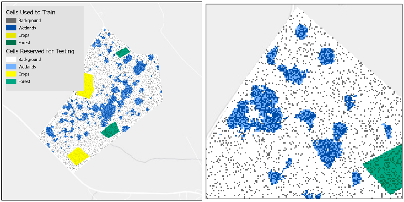
Training and testing rasters created from a multiclass groundtruth raster and varying sampling percentages
Results Interpretation and Model Development
Developing a wetland model that is best suited to your target landscape and application will be an iterative process informed by results interpretation. The entire suite of accuracy metrics generated should be considered when evaluating model performance. In assessing the performance of a model, consider:
The difference in true negative rate (nonwetland recall) and true positive rate (wetland recall) in an imbalanced area. In an area where true wetlands are very sparse, a high true negative rate, low true positive rate, and high overall accuracy can be misleading. Consider that in an area where there is much more nonwetland area than wetland - an unskilled model could predict the entire area to be nonwetland and achieve "high" overall accuracy while identifying 0% of the wetlands.
The tradeoff between wetland recall and precision. Unless you have a very high performing model, you can expect precision to decrease as recall increases. This is because more predictions need to be made to increase recall, and this typically results in some erroneous predictions (i.e., lower precision) as well. When you are past the point of being able to increase both metrics, you should consider whether it is more costly to omit true wetlands (related to recall) or overpredict wetlands (related to precision). Balancing these metrics can be accomplished through model development or using the probability raster to explicitly define the confidence threshold required to make a wetland prediction.
The precision-recall (PR) curve as a way to summarize model performance. The PR curve shows the precision and recall for that specific class if class predictions were made at varying confidence thresholds. The area under this curve, or Average Precision (AP), summarizes model performance for identifying that specific class, with values closer to 1 indicating a better model. When the AP score gets closer to 1, it shows that as the confidence threshold is lowered and the model makes more predictions for that class, recall increases with minimal sacrifice to precision/overprediction.
Moreover, ways to improve your model may include:
Alternative training sampling schemes. Literature supports undersampling the majority class in an imbalanced scenario can improve the detection rate of the minority class. In other words, you may want to sample less of nonwetland class(es) if they represent a much larger proportion of your entire project area compared to the wetland class.
Remove the training constraint or change its location. It is possible that the wetlands found within the training constraints are not representative of the types of wetlands in the testing area. By sampling more types of wetlands, the model can learn a more robust set of wetland characteristics.
Experiment with additional trials of the DEM preprocessing phase. Literature shows that the best performing smoothing method and scale for the DEM may vary between the topographic predictor variables. Also, depending on the size of wetlands typical to the target area, predictor variables may model the wetland hydrology better when derived at coarser or finer scales.
Improve the quality of the ground truth datasets. It is important to be confidence in the spatial extents to which you know wetland coverage. Otherwise, it is possible that additional wetlands exist in the ground truth dataset and the model could be trained and assessed on incorrect data. Further, model results may improve with more discrete and unique classes in the ground truth data IF the predictor variables used are good distinguishers between the classes. Improving the quality of this data would not only improve the model training, but also provide a more representative accuracy assessment.
Include additional predictor variables. The baseline, topographic predictor variables included with WIM have been shown to be useful for wetland mapping across landscapes. However, they are not at all exhaustive of relevant landcover characteristics. If additional predictor variables are available for your project area, they should be included in your model development iterations. Presumably, including vegetative information or other imagery-based data would improve results. These additional predictors may be especially helpful in areas with few topographic variations or with coastal or glacial subsurface influence. It is important to keep in mind, however, that the same set of predictor variables must be present for any other area that you want to apply your trained model to.
Individual Tool Help
See the documentation for tool metadata. Relevant notes beyond Tool Metadata, if any, follow.
Preprocess Ground Truth Data
Algorithm Notes:
See usage examples below.
Smooth High-Resolution DEM
Algorithm Notes:
Execution of Gaussian smoothing in the WIM is based on code from Sangireddy et al. (2016).
Execution of Perona Malik smoothing in the WIM is based on code from Sangireddy et al. (2016).
Calculate Depth to Water Index using Surface Parameters
Algorithm Notes:
This tool calculates the cartographic depth-to-water index (DTW) to be subsequently used as a predictor of wetland areas. The DTW, developed by Murphy et al. (2007), is a soil moisture index based on the assumption that soils closer to surface water, in terms of distance and elevation, are more likely to be saturated. Calculated as a grid, the DTW is defined as
| (1) |
|---|

where dz/dx is the downward slope of cell i along the least-cost (i.e., slope) path to the nearest surface water cell, a is a factor accounting for flow moving parallel or diagonal across pixel boundaries, and xc is the cell resolution (Murphy et al., 2007). The WIM implementation of eq. (1) requires two inputs: a slope raster to represent the cost surface and a surface water raster to represent the source location.
The tool performs the following actions:
Calculates a DTW-specific slope raster from the input DEM unless one is provided as an optional input.
Optionally saves the intermediate outputs created during processing.
Creates the DTW raster using the surface water raster as the source and the DTW slope raster as the cost.
Calculate Curvature using Surface Parameters
Algorithm Notes:
Calculate Topographic Wetness Index using Surface Parameters
Algorithm Notes:
This tool calculates the topographic wetness index (TWI) to be subsequently used as a predictor of wetland areas. The TWI relates the tendency of an area to receive water to its tendency to drain water, and is defined as
| (2) |
|---|

where a is the specific catchment area (contributing area per unit contour length) and tan(B) is the local slope (Beven & Kirkby, 1979). The WIM implementation of eq (2) requires a TWI slope and specific catchment area as inputs, although both can be calculated directly from the input high-resolution DEM.
The tool performs the following actions:
Calculates a TWI-specific slope raster from the input DEM, unless one is provided as an optional input.
Calculates a specific catchment area raster from the input DEM, unless one is provided as an optional input.
Optionally saves the intermediate outputs created during processing.
Creates the TWI raster by implementing eq. (2) as a raster algebra expression.
Train Test Split
Algorithm Notes:
Train Random Trees
Algorithm Notes:
This tool executes the training phase of the Random Trees algorithm. In this phase, the algorithm takes bootstrap samples of the training dataset, including the labeled cells in the training raster and the predictor variables. A decision tree is created from each bootstrap sample, and all are used to learn the indicators of the ground truth classes based on information from the predictor variables. In doing this, the Random Trees algorithm is less susceptible to overfitting. This tool uses the Scikit-Learn Python library (Scikit-Learn Developers, 2017a) to execute the Random Trees algorithm. For a more detailed discussion of the algorithm and its fit for WIM, see O'Neil et al. (2019).
The tool performs the following actions:
Prepares the predictor variable raster(s) for use by the Scikit-Learn library. If more than one predictor variable raster is given, a composite raster is created from all input predictor variables and saved to the Prepared Predictor Variable Raster name. If only one raster is passed, it will be copied and saved to the Prepared Predictor Variable Raster name, but it can be disregarded for later steps. In either case, the cells in the prepared raster are extracted only where the training labels before further use.
Initializes the Random Trees model according to the number of trees, the maximum tree depth, the maximum number of features, and the class weights. If users omit these parameters or leave them unaltered, default values are used. Users should see Scikit-Learn documentation for further details on these parameters (Scikit-Learn Developers, 2017a).
Trains the initialized model given the training dataset. Saves the trained model to a JOBLIB file.
Saves the variable importance measures to a TXT file. These measures provide an estimate of the decrease in accuracy of the model if that predictor variable was removed.
Common Error Messages:
Generic error due to Composite Bands tools on the backend
Fix - Open the Composite Bands geoprocessing tool, navigate to its environment settings, change the Parallel Processing Factor to 0, re-run the Train Random Trees tool.
Or, after changing the Parallel Processing Factor, run the Composite Bands tool directly where the input rasters will be the same list of rasters that were entered into the predictor variables raster list. The output composite raster will be used as the only input predictor variables raster in the Train Random Trees tool. A copy of the composite raster will be created by the Train Random Trees tool, this can be ignored. Continue with the rest of the workflow.
IndexError: boolean index did not match indexed array along dimension 0; dimension is XXXX but corresponding boolean dimension is XXXX
This error is due to a mismatch in raster extents between the prepared predictior variable raster (the composite raster of the list of predictor variable rasters entered, or the single predictor variable entered if only one is being used) and the training raster. On the backend, the tool attempts to clip the prepared predictor variable raster to the same extents as the training raster. This error indicates that this process has failed.
As a workaround, try:
Manually run Composite Bands on the predictor variable rasters (or proceed with the single predictor variable raster being used)
Manually run Clip Raster between the result and the training raster
Check in the raster properties that the number of columns and rows is the same as those in the training raster
Also consider that the training raster must fit entirely within the extents of the predictor variables being used. If the training raster extends beyond, generate the predictor variables for entire extent of the area, or use a smaller ground truth area if the prior is not possible.
"ValueError: Input contains NaN, infinity or a value too large for dtype('float32')."
This error indicates that one of your Predictor Variable Rasters has a pixel type larger than 32 bit and/or a No Data value of NaN. On the backend, the scikit-learn library is used and has a value limitation that is exceeded by NaN values. This error source can be confirmed by opening the raster properties of a raster and seeing the No Data value and the pixel type parameters.
This error is more common if one of the rasters were created outside of ArcGIS Pro or with tools other than WIM tools.
For each of the rasters with NaN as the No Data value and/or pixel type of 64 bit
Run Copy Raster
Specify the output to be a TIFF
Specify the Pixel Type to be 32 bit signed
Choose a No Data Value other than nan
A common No Data value for 32 bit rasters is -3.4028235e+38
After running once, you may see that most of the raster is black and the minimum value is very large (e.g., -20000000). This will not interfere with further processes, but you can re-run Copy Raster with this unrealistic minimum value as the No Data Value parameter.
Run Random Trees
Algorithm Notes:
This tool uses the trained Random Trees model to predict the class for the cells of the input predictor variables. Predictions do not need to be made in the same area for which the model was trained, but the calculation of the predictor variable(s) must be the same. In this case, a model can be trained using the DTW, Curvature, and TWI for one area and used to make predictions for a new area, if DTW, Curvature, and TWI have also been derived and are used as inputs.
The tool performs the following actions:
Loads the JOBLIB model and uses it to predict wetland and nonwetland areas for the predictor variables raster. Internally, the random trees algorithm uses the relationships learned between the predictor variables and class values during training and determines the final predicted class based on the majority vote of all decision trees created.
If "Save probability rasters" is True, uses the JOBLIB model to produce the probability raster for each target class (e.g., wetland and nonwetland). The values in these rasters represent the probability that the cell belongs to the class in question on a 0-1 scale. These outputs can be useful for decision makers where the tradeoff between wetland detection and overprediction can be examined. Producing and saving these outputs also allow for a more thorough accuracy assessment in later steps.
Assess Accuracy
Algorithm Notes:
Given the predicted output from a supervised classification model and labeled ground truth data (i.e., the testing raster), a report is generated summarizing the performance of the model for the locations of the testing data (ideally, locations not used for training the model). Additional metrics are generated if the user includes output class probability rasters. Accuracy metrics were chosen to avoid misleading assessments of imbalanced ground truth classes, which is typical of wetland/nonwetland distributions. For further details and justification for the metrics chosen, see O'Neil et al. (2019). Accuracy metrics are calculated using the Scikit-Learn library (Scikit-learn Developers, 2017b). Inputs and outputs are shown in the example run.
The tool performs the following actions:
Creates a new directory for accuracy metrics if the specified one does not already exist.
If necessary, extracts the prediction raster cells that overlap with the testing raster cells.
Calculates and plots a confusion matrix. The confusion matrix categorizes each cell (represented in units of km2 and m2) into one of four groups: true positive, true negative, false positive, or false negative. These categories indicate that the predicted cell either correctly identified wetland area, correctly identified nonwetland area, incorrectly identified a wetland area, or incorrectly identified a nonwetland area, respectively. The plots are saved as PNG files to the accuracy metrics directory as "conf_matrix" and "conf_matrix_meters."
Creates a classification report and saves to a TXT file as "summary_stats." For each class, this report gives the precision, recall, f1-score, and support. Although metrics are calculated for each class, the descriptions below focus on the interpretation of scores for the wetland class. Note that other metrics given by the classification report may be misleading for imbalanced class predictions. For more information on these, users should see the Scikit-Learn documentation (Scikit-learn Developers, 2017b).
Precision is a metric that accounts for overprediction of the positive class (i.e., wetlands), without being biased by disproportionately large populations of the negative class (i.e., nonwetlands). Precision is the percentage of wetland predictions made that were correct, calculated as:
| (3) |
|---|

Recall is a metric of class detection, giving the percentage of true wetlands that were correctly identified:
| (4) |
|---|

F1 score represents a weighted average of precision and recall, where the best F1 score is a value of 1 and a worst score is a value of 0. It is important to note that this metric assumes that high detection rate and low overprediction are equally important to stakeholders. Other forms of the F1 score exist where these components can be given different weights. The F1 score is defined as
| (5) |
|---|

Finally, support represents the total samples (number of cells) in the true wetland class.
- If class probability rasters are passed, calculates and plots precision-recall curves for each probability raster, which each corresponds to a single class, given. Precision-recall curves plot precision versus recall for each predictive threshold of that class. That is, the curve will show the precision and recall scores if each cell required 0-100% probability of belonging to a class before being assigned to that class. In addition, the Average Precision score is calculated for each precision-recall curve. Average Precision is a surrogate for the area under the precision-recall curve, and it is used to summarize model performance for the class of interest. An Average Precision score closer to 1 indicates a better performing model. The Average Precision metrics is calculated as,
| (6) |
|---|

Where Pn and Rn are the precision and recall at the nth predictive threshold, respectively.
References
Beven, K. J., & Kirkby, M. J. (1979). A physically based, variable contributing area model of basin hydrology. Hydrological Sciences Journal, 24(1), 43-69. https://doi.org/10.1080/02626667909491834
Moore, I. D., Grayson, R. B., & Ladson, A. R. (1991). Digital terrain modelling: a review of hydrological, geomorphological, and biological applications.Hydrological processes,5(1), 3-30. https://doi.org/10.1002/hyp.3360050103
Murphy, P. N., Ogilvie, J., Connor, K., & Arp, P. A. (2007). Mapping
wetlands: a comparison of two different approaches for New Brunswick,
Canada.Wetlands,27(4), 846-854.
https://doi.org/10.1672/0277-5212(2007)27\[846:MWACOT\]2.0.CO;2]27%5b846:MWACOT%5d2.0.CO;2)
O'Neil, G. L., Goodall, J. L., & Watson, L. T. (2018). Evaluating the potential for site-specific modification of LiDAR DEM derivatives to improve environmental planning-scale wetland identification using Random Forest classification.Journal of hydrology,559, 192-208. https://doi.org/10.1016/j.jhydrol.2018.02.009
O'Neil, G. L., Saby, L., Band, L. E., & Goodall, J. L. (2019). Effects of LiDAR DEM smoothing and conditioning techniques on a topography-based wetland identification model.Water Resources Research, 55,4343-4363. https://doi.org/10.1029/2019WR024784.
O'Neil, G. L., Goodall, J. L., Behl, M., & Saby, L. (2020). Deep learning using physically-informed input data for wetland identification. Environmental Modelling & Software, 126, 104665.
Passalacqua, P., Do Trung, T., Foufoula-Georgiou, E., Sapiro, G., & Dietrich, W. E. (2010). A geometric framework for channel network extraction from lidar: Nonlinear diffusion and geodesic paths. Journal of Geophysical Research, 115, F01002. https://doi.org/10.1029/2009JF001254.
Sangireddy, H., Stark, C. P., Kladzyk, A., & Passalacqua, P. (2016). GeoNet: An open source software for the automatic and objective extraction of channel heads, channel network, and channel morphology from high resolution topography data. Environmental Modelling & Software, 83, 58-73. https://doi.org/10.1016/j.envsoft.2016.04.026.
Scikit-learn Developers. (2017a). Ensemble Methods. Retrieved August, 2018 from http://scikit-learn.org/stable/modules/ensemble.html\#forest
Scikit-learn Developers. (2017b). Model evaluation: quantifying the
quality of predictions. Retrieved August 2018, from
http://scikit-learn.org/stable/modules/model\_evaluation.html