Identifying Wetlands with Deep Learning
Download the PDF here
Introduction
The Wetland Identification Model (WIM) employs the Random Trees (forests) algorithm to predict wetlands. Random Trees has several advantages over other machine learning methods, including its ability to incorporate both continuous (e.g., raw elevation values, topographic indices) and categorical (e.g., geomorphology landform classifications) data and its ability to reach higher accuracy with less training data as a result of bootstrapping.
However, the Random Trees algorithm is typically limited in the quantity of training data it can incorporate because it ingests data as NumPy arrays. Random Trees also are not able to consider the spatial context of predictor variables. In the case of wetland identification, where the target classification object is a cohesive geomorphologic object, this is a significant failing since areas that "look" like a wetland are even more likely to be a wetland when its neighbors also "look" like wetlands.
Deep Learning emerges as an attractive alternative to address these shortcomings. Implemented through tensor data objects, Deep Learning implementations can inherently ingest significantly more training data and predictor variables than Random Trees or other machine learning frameworks. Another feature of Deep Learning frameworks is their ability to further train models, starting from a checkpoint of a pre trained model (i.e., fine-tuning). This allows for the opportunity to improve models over time as more training data is collected and/or more nuanced instances of a target classification is identified.
While Deep Learning implementations entail additional overhead as far as data preparation and allocating computing resources, improvements to wetland predictions can be too good to pass up! Esri technology streamlines Deep Learning implementations for GIS data. Arc Hydro's WIM tools can be used in conjunction with core Esri Deep Learning tools to allows users to develop, assess, and deploy custom Deep Learning models to meet specific use-cases.
Continue reading for an example workflow that leverages WIM tools within an Esri Deep Learning workflow to predict wetlands. Our example is based off a collaborative effort with the National Wetland Inventory (NWI) and State of Minnesota to evaluate WIM's potential to identify wetlands in low-lying regions using Deep Learning.
New to Deep Learning? Check out these Esri resources!
Step 1 - Prepare Ground Truth Data
Our specific use case works from ground truth data delineated for disparate plots across a landscape in Minnesota. Since we are working with multiple ground truth scenes, rather than a single, contiguous ground truth area, additional preprocessing is necessary. Additionally, because our data is not created with the Training Sample Manager, we must manually edit the schema to comply with requirements of Export Training Data for Deep learning. Note that in cases with a single, contiguous area of training data, users should specify a single target class (i.e., "wetland") and the Deep Learning model will assign the remainder of the area as background/NoData.
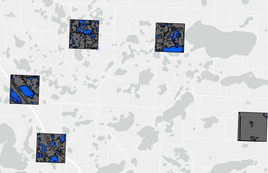
Figure 1. Raw ground truth scenes where ground area is delineated only within the extents of individual chips. Each chip contains multiple wetland polygons (blue).
- Dissolve the individual wetland polygons within each chip to convert contiguous wetlands into single features.
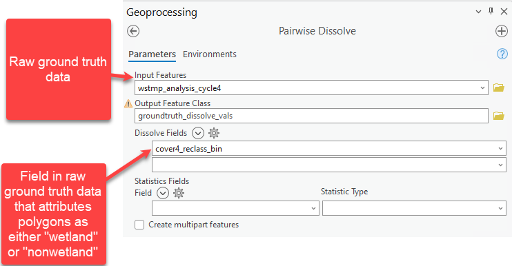
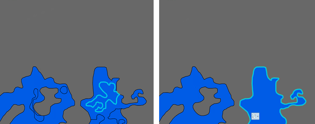
Figure 2. Single wetland selected before (left) and after (right) dissolving.
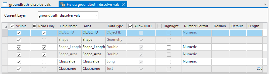
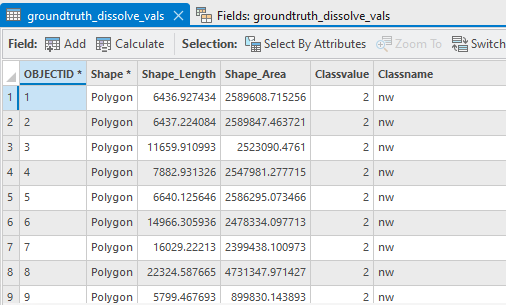
- Modify the feature class schema to contain only two attributes: "Classvalue" and "Classname". "Classname: will be the plain text representation of the target prediction classes and "Classvalue" will be the integer representation.
- Prepare the extents feature class to ensure Deep Learning training chips are only created within the individual ground truth scenes. Use Dissolve again, but do not specify a dissolve field. This will result in each training scene becoming a single feature itself. The resulting feature class will be used as the Input Mask Polygons in Step 2.
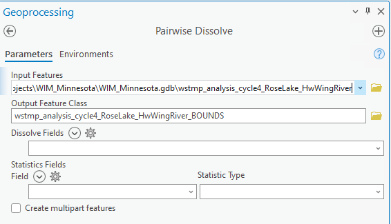
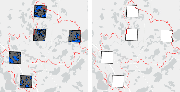
Figure 3. Prepared ground truth scenes within the HUC of interest (left) and the accompanying extents for those scenes (right).
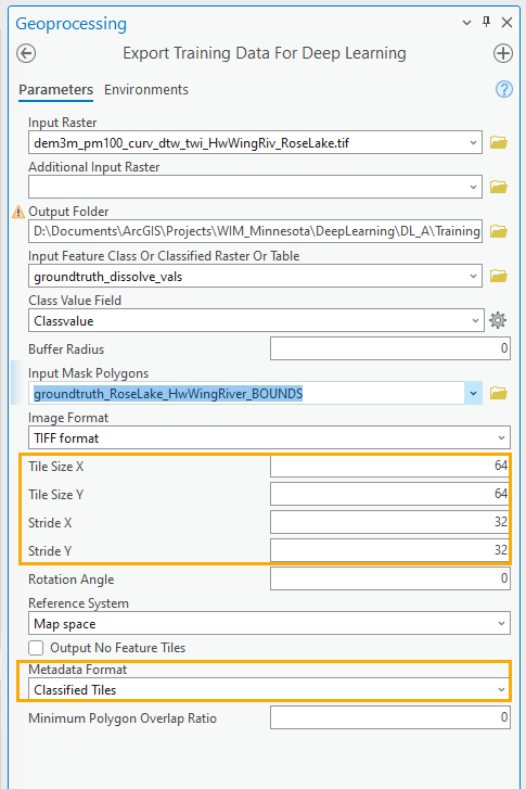
Step 2 - Export Training Data
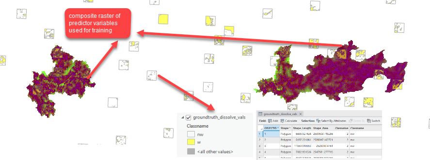
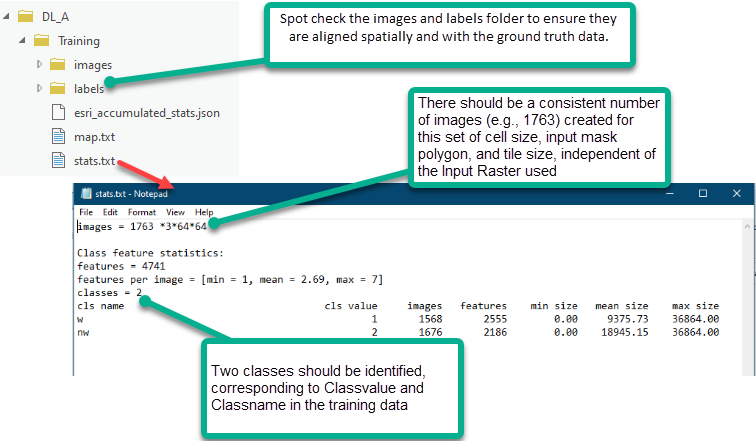
Use Export Training Data for Deep Learning to subdivide your training dataset into training chips that the [arcgis.learn] Deep Learning models can consume. In addition to the ground truth data prepared in Step 1, you will use an Input Raster that contains the predictor variables the model will learn from. The Input Raster must 1) be in the same projection as the ground truth data, and 2) overlap with the ground truth data. If your model will learn from more than one predictor variable, use the Composite Bands tool to combine the multiple predictor variables into a single, multidimensional raster. The result of this operation will be a training dataset directory that contains training chips within the Input Mask Polygon. Each training chip consists of a predictor variable chip and accompanying label (ground truth coverage) chip. The model configuration we are using (UNet) will automatically normalize predictor variable data. However, this may not be true for other model configurations and users should confirm this detail in their own workflows.
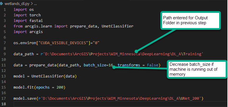
Step 3 - Training
With your prepared training dataset, you can now train the Deep Learning model. We will apply a UNet model architecture. It is recommended that your machine has adequate GPU resources for the training and inferencing steps.
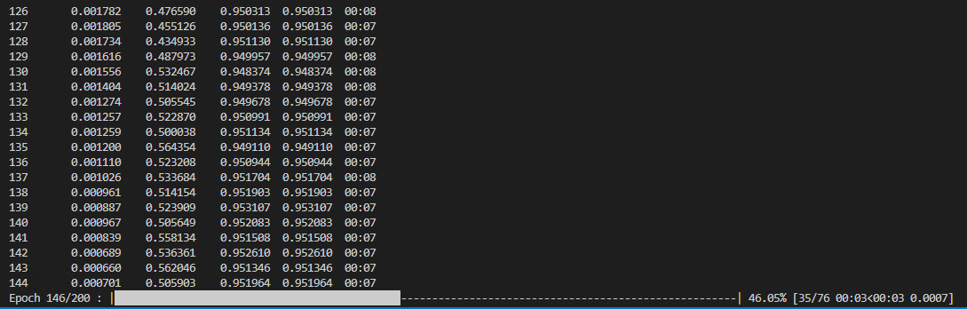
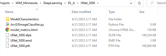
When training is complete, the trained model (saved as *.emd and *.dlpk) and training metrics are available in the specified model save location.
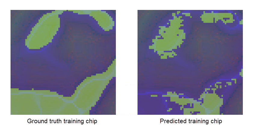
The model metrics file shows the changes in training and validation losses during training epochs. It also shows previews of the labeled training chip and the model's prediction for that same area.
Step 4 - Inference
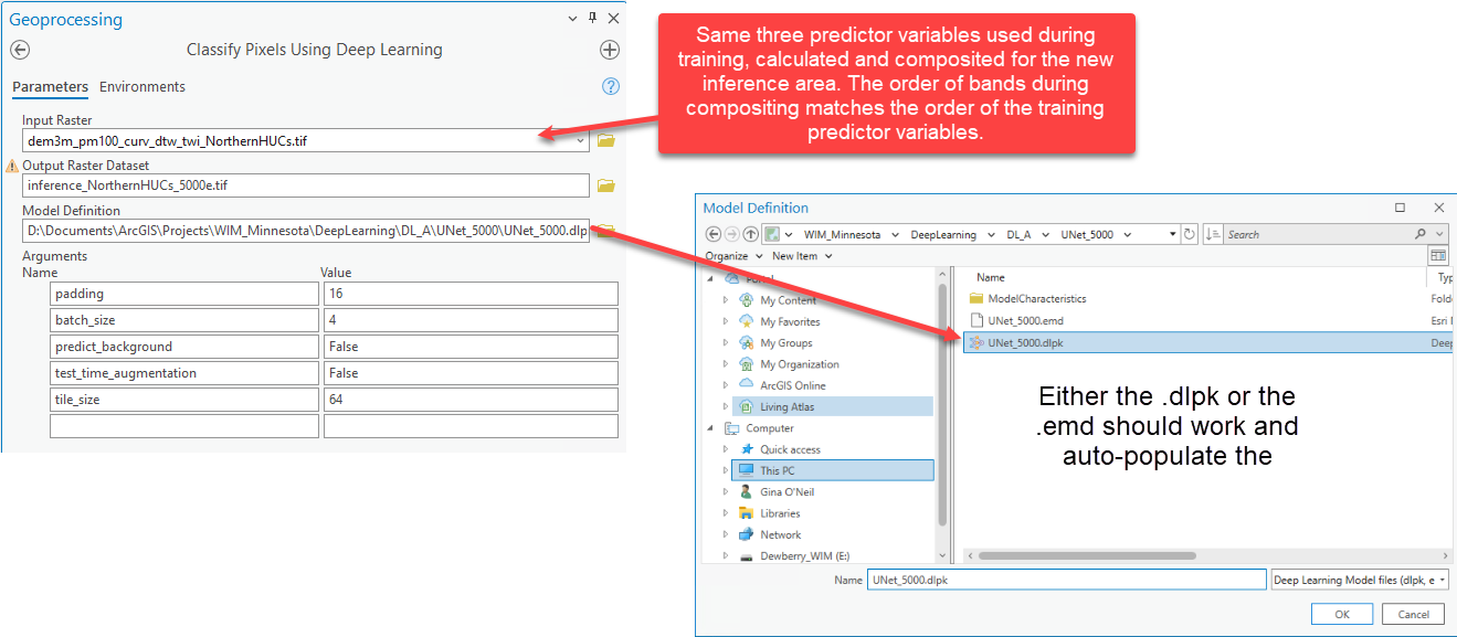
You can now apply your trained model to other areas to generate predictions. The trained model is trained specifically to identify wetland vs. nonwetland using the combination of predictor variables used during training. Inferencing for a scenario different from the training configuration will result in poor performance and/or tool errors. To inference for targets other than those specified in your original ground truth data, you will need to fine-tune the model by training it further for those new targets. To inference with a different combination of predictor variables, you will need to train an entirely new model.
In the example below, we are inferencing in a new area. We created the same predictor variables in the inference area as were created in the training area. The inference area predictor variables were then combined in the same order as was used in the training area, using the Composite Bands tool.
The output inference raster will have pixel values for one of the prediction targets. The sample results shown below render the predicted wetland pixels as blue and the predicted nonwetland pixels as no-color. We can visually assess our results at a high level by comparing them to Living Atlas imagery.
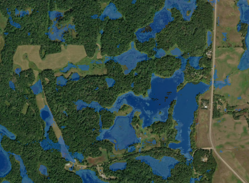
Figure 5. Sample inference results with predicted wetlands shown in blue and predicted nonwetlands shown as no-color.
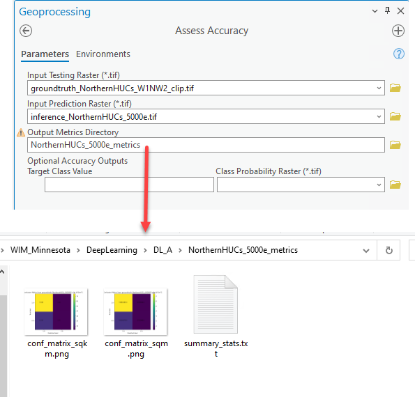
Step 5 - Accuracy Assessment
There are several methods for calculating the accuracy of your predictions. Regardless of the chosen method, accuracy assessments are representative of model performance if they are completed in areas where your model did not train. You will need model predictions and verification data (i.e., additional ground truth data) in an area where the model was not trained. Metrics are then calculated based on how frequently a prediction aligns with the verified land cover. The resulting accuracy metrics are only valid for the area covered by the verification data, but they can represent the expected accuracy in similar areas.
To complete an accuracy assessment with the WIM Assess Accuracy tool, you will need an integer raster representation of verification data where the raster has the same cell size and extents as the inference raster. This can be accomplished with the WIM Preprocess Ground Truth Data tool, plus an additional check.
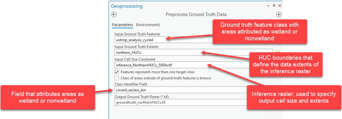
- Preprocess Ground Truth Data
- Confirm the integer representation of prediction targets are the same as what was used during training. We have mismatched encoding that we will address in the next step.
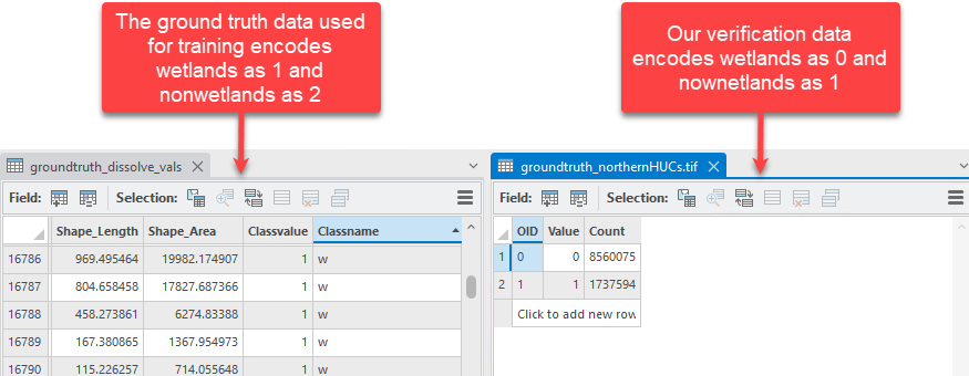
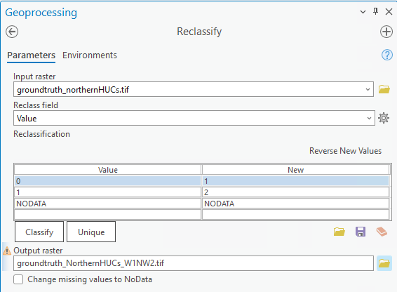
- Use Reclassify (Spatial Analyst) to recode wetlands as 1 and nonwetlands as 2. This will ensure the proper comparison of pixel values between the inference raster and the verification data.
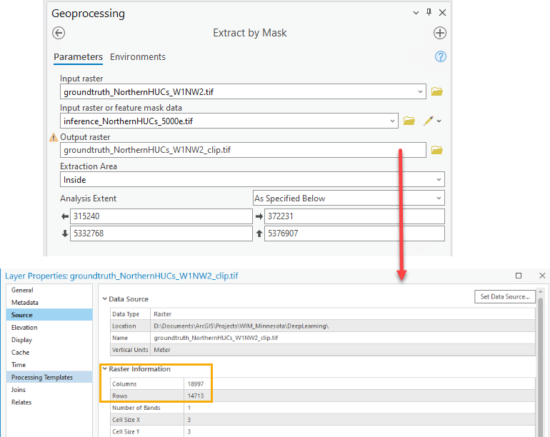
- Check if the verification raster has the same number of columns and rows as the inference raster. If they do not, you can take an additional step to force the extents to be the same.
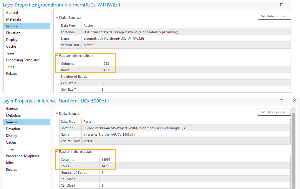
- Use Extract By Mask to achieve the same columns and rows between verification and inference rasters.
- We are now ready to use Assess Accuracy. This tool will summarize results using a confusion matrix, calculating the Precision and Recall per prediction target.