Concepts#
Core concepts for working with Geometry in Big Data Toolkit’s Processors and Functions.
Shape Column#
Shape is stored as a struct for easier handling and processing. The struct is composed of WKB, XMIN, YMIN, XMAX, and YMAX values. Transform Shape struct to WKT before persisting to csv. Parquet can store the Shape struct without additional transformation.
spark.sql("SELECT ST_MakePoint(-47.36744,-37.11551) AS SHAPE").printSchema()
root
 |-- SHAPE: struct (nullable = false)
 |    |-- WKB: binary (nullable = true)
 |    |-- XMIN: double (nullable = true)
 |    |-- YMIN: double (nullable = true)
 |    |-- XMAX: double (nullable = true)
 |    |-- YMAX: double (nullable = true)
df = (spark
   .read
   .format("com.esri.spark.shp")
   .options(path="/data/poi.shp", format="WKB")
   .load()
   .selectExpr("ST_FromWKB(shape) as SHAPE")
   .withMeta("Point", 4326))
df.selectExpr("ST_AsText(SHAPE) WKT").write.csv("/tmp/sink/wkt")
+---------------------------+
|WKT                        |
+---------------------------+
|POINT (-47.36744 -37.11551)|
+---------------------------+
Shape structs can be created using multiple methods:
Processors
Functions
Shape structs can be exported. Use these methods to transform Shape structs into formats suitable for data interchange:
Metadata#
Metadata is set for the dataframe and describes the Geometry column. The metadata specifies the geometry type, spatial reference (wkid), and the name of the column. Metadata is required to use Processors on your dataframes but not required for BDT’s Python functions or SQL expressions. Similarly, Processors return dataframes with metadata set while Functions do not. The default column name is SHAPE if not specified when adding metadata. Parquet may persist metadata but must always be specified
when reading other sources like csv. As a best practice always specify the metadata so geometry type and spatial reference are clear to the reader. Unlike other processors, ProcessorAddMetadata can be called on the dataframe df2 = df1.withMeta("Point", 4326)
Spatial reference is a key part of metadata. See https://spatialreference.org/ for more detailed information about available spatial references.
# Python
df1 = (spark
    .read
    .format("csv")
    .options(path="/data/taxi.csv", header="true", delimiter= ",", inferSchmea="false")
    .schema("VendorID STRING,tpep_pickup_datetime STRING,tpep_dropoff_datetime STRING,passenger_count STRING,trip_distance STRING,pickup_longitude DOUBLE,pickup_latitude DOUBLE,RatecodeID STRING,store_and_fwd_flag STRING,dropoff_longitude DOUBLE,dropoff_latitude DOUBLE,payment_type STRING,fare_amount STRING,extra STRING,mta_tax STRING,tip_amount DOUBLE,tolls_amount DOUBLE,improvement_surcharge DOUBLE,total_amount DOUBLE")
    .load()
    .selectExpr("tip_amount", "total_amount", "ST_FromXY(pickup_longitude, pickup_latitude) as SHAPE")
    .withMeta("Point", 4326, shapeField = "SHAPE"))

df1.schema[-1].metadata
{'type': 33, 'wkid': 4326}
QR, RC, and Cell size#
QR is the spatial partitioning mechanism used by BDT. QR and RC are functionally equivalent. RC will be deprecated in a future release, with QR fully adopted moving forward.
Cell size sets the size of each QR, and therefore the size of each spatial partitioning grid cell. It is specified in the units of the spatial reference e.g. degrees for WGS84, meters for Web Mercator. Cell size is an optimization parameter used to improve efficiency of processing and is based on your data size and distribution, size of the cluster, and analysis workflow. If you are working with polygons start with a cell size that is one standard deviation larger than the mean area of each
polygon in the set. Cell size will be ignored when setting doBroadcast = True in the processor.
points_in_county = bdt.processors.pip(
    points,
    county,
    cellSize = 0.1,
)
Note: Cell size must not be smaller than the following values:
For Spatial Reference WGS 84 GPS SRID 4326: 0.000000167638064 degrees
For Spatial Reference WGS 1984 Web Mercator SRID 3857: 0.0186264515 meters
Spatial partitioning can be performed using SQL. The following example shows how to use QR for spatial partitioning using SQL. It assumes the incoming DataFrames have an ID column and a SHAPE column.
ldf_qr = ldf.select("LID", "SHAPE", explode(F.st_asQR("SHAPE", cellSize)).alias("QR"))
rdf_qr = rdf.select("RID", "SHAPE", explode(F.st_asQR("SHAPE", cellSize)).alias("QR"))

ldf_qr.createOrReplaceTempView("lhsDF")
rdf_qr.createOrReplaceTempView("rhsDF")

expectedDF = spark.sql(
    f"""
    SELECT LID, lhsDF.SHAPE AS LHS_SHAPE, RID, rhsDF.SHAPE AS RHS_SHAPE
    FROM lhsDF
    LEFT JOIN rhsDF
    ON lhsDF.QR == rhsDF.QR
    AND ST_IsLowerLeftInCell(lhsDF.QR, {cellSize}, lhsDF.SHAPE, rhsDF.SHAPE)
    """)
This can also be done using the join_qr processor. This processor Spatially indexes the data, which will accelerate joins significantly on very large DataFrames. On smaller DataFrames, the overhead incurred from spatially indexing the geometries is greater than the speed benefit. For reference, benefit was not seen until each DataFrame exceeded 20 million records.
This processor will calculate QR internally if there is not already a QR column provided in the input DataFrames. It is recommended to let the processor calculate the QR internally as it takes advantage of internal optimizations to avoid unnecessary spilling.
The join_qr processor accepts join_distance as a parameter. Features within this distance will be joined together. Setting join_distance to 0 enforces feature-to-feature touches and intersection conditions in downstream operations. If distance or nearest operations will be run downstream after the join, then set the distance value in join_qr to the same distance value that will be used later on in those functions.
The following example shows the recommended way to perform spatial partitioning using the join_qr processor.
import bdt.processors as P

cellSize = 0.1
joinDistance = 0.0

ldf = spark.createDataFrame([ \
        ("POLYGON ((1 1, 2 1, 2 3, 4 3, 4 1, 5 1, 5 4, 1 4, 1 1))",),], schema="WKT1 string") \
        .selectExpr("ST_FromText(WKT1) AS SHAPE") \
        .withMeta("POLYGON", 4326)

rdf = spark.createDataFrame([ \
        ("POLYGON ((1 1, 5 1, 5 2, 1 2, 1 1))",),], schema="WKT1 string") \
        .selectExpr("ST_FromText(WKT1) AS SHAPE") \
        .withMeta("POLYGON", 4326)

## run an inner join
joined_df = P.join_qr(
                ldf,
                rdf,
                join_type="inner",
                cell_size = cellSize,
                join_distance = joinDistance)
Cache#
Caching a DataFrame is a Spark optimization technique that can increase the performance of your workflows. The cached DataFrame is saved in memory and spilled to disk if needed.
If a DataFrame is being used multiple times in a workflow, then caching can speed up the workflow. However, be careful about memory management.
Calling the DataFrame cache method on the output DataFrame returned by a BDT processor is the same as setting
cache = truein the processor parameters. Note:cacheas a processor parameter is being deprecated in future releases.See the below code for an example of how caching could be used in the context of a workflow.
# Python

# Read a parquet file of point geometries.
points = spark \
    .read \
    .parquet("/path/to/points.prq")

# cache the point dataset
points.cache()

# create spark logical and physical plans for pip
points_in_county = bdt.processors.pip(
    points,
    county,
    cellSize = 0.1)

# the .cache() on the point DataFrame will be lazily evaluted on this write operation...
points_in_county \
    .write \
    .parquet("/path/to/output_countypoints.prq")

points_in_zip = bdt.processors.pip(
    points,
    zip_codes,
    cellSize = 0.1)

# ... and assuming that the "zip_codes" DataFrame is about the same size as the "county" DataFrame,
# this write will take much less time since the point DataFrame was cached in the previous write operation.
points_in_zip \
    .write \
    .parquet("/path/to/output_zippoints.prq")
Extent#
An array of xmin, ymin, xmax, ymax that contains the spatial index.
In units of the spatial reference e.g. degrees for WGS84, meters for Web Mercator, etc.
Defaults to World Geographic SRID 4326 [-180.0, -90.0, 180.0, 90.0]
IMPORTANT: When using a projected coordinate system, the extent must be specified. For example, if the data is in Web Mercator SRID 3857, then an extent must be specified in 3857.
Try to tailor the extent for the data to reduce processing of empty areas and improve performance.
The Extent Helper Application is useful for defining an extent in Web Mercator.
LMDB#
The LMDB (Lightning Memory-Mapped Database) is a database that holds all street network information required for certain processors and functions. You will need an appropriate license to Street Map Premium and a prebuilt LMDB file provided by the BDT Support team.
The LMDB is only supported on Databricks. It is deployed to every node on the Databricks cluster with an init script. For example, the below init script will download and copy the LMDB to the workers:
#!/usr/bin/env bash

mkdir /data

#Download AzCopy
wget https://aka.ms/downloadazcopy-v10-linux

#Expand Archive
tar -xvf downloadazcopy-v10-linux

#Move azcopy onto path
sudo cp ./azcopy_linux_amd64_*/azcopy /usr/bin/

# LMDB
azcopy copy 'https://<mystorageaccount>.blob.core.windows.net/<mystoragecontainer>/LMDB/LMDB_3.0_2021_R3_Q2?<SAS_TOKEN>' '/data' --recursive=true
then set the spark properties:
spark.bdt.lmdb.map.size 304857600000
spark.bdt.lmdb.path /data/LMDB_<version>_<year>_<quarter>
Processors that Require LMDB:
SQl Functions that Require LMDB:
When using these processors and functions it is advised to use a cluster with many smaller machines (fewer cores) rather than a few large machines with many cores per machine. This is because it is possible to reach an LMDB readers full exception where there are too many processes using the LMDB on one machine. Using more machines will create an LMDB for each machine and the data will be distributed across more LMDBs than if there were fewer machines. It is also advised to choose a worker
type with at least 128GB of memory to accomodate for the size of the LMDB.
The LMDB is updated yearly with the new Street Map Premium data, and certain versions are compatible with certain versions of BDT3.
BDT Version |
LMDB Version |
|---|---|
BDT3 3.0 |
LMDB_3.0_2021_R3_Q2 |
BDT3 3.1 |
LMDB_3.1_2022_R2 |
BDT3 3.2 |
LMDB_3.2_2023_R2 |
BDT3 3.3 |
LMDB_3.3_2023_R4 |
BDT3 3.4 |
LMDB_3.4_2024_R2 |
Geometry Acceleration#
Geometry acceleration is a parameter that can be tuned to increase the performance of operations that use the same geometry many times.
This parameter can be set to none, mild, medium, or hot. Mild acceleration uses some memory and time up front to speed up operations done on the same geometry many times. Meanwhile, hot provides the most acceleration using more memory and time up front but potentially resulting in greater speedups if the geometry is used many times. None performs no acceleration.
In most scenarios, acceleration is not beneficial. Hence, the default acceleration for most functions that can accelerate geometries is none. However, there are certain cases where it may provide a speedup.
When to accelerate:
If you are dealing with a large polygon or a polyline that participates in the same operation many times over.
If you are taking advantage of broadcasting. Because broadcasting may distribute a single geometry to many partitions, the geometry may be used in a similar operation on each partition.
If you are using the raster processors tabulate_area or zonal_statistics_table. These processors may use an input geometry many times depending on the size of the raster. The default acceleration for these functions is mild.
Large Polygons#
Large polygons and multipolygons can slow down BDT processes. There are several ways to identify if your dataset has a large polygon:
You have a small dataset but your process is taking a long time.
A task in your process is hanging.
Executor loss is observed in the SparkUI.
A polygon in your dataset has a high number of vertices.
A polygon in your dataset has a large or very small (possibly negative) area.
The extent of a polygon in your dataset spans a large area.
Invalid polygons can become very large when projected or simplified. Consider checking your dataset for invalid polygons using ST_IsValid along with the above conditions before/after simplification and before/after projection.
In the case of a large single polygon, considering clipping the polygon into smaller pieces. ST_Chop1, 2, or 3, as well as ST_Dice can also be used to break a polygon into smaller pieces.
Multipolygons with a large extent and lots of negative space can cause similar issues. See the example multipolygon below:
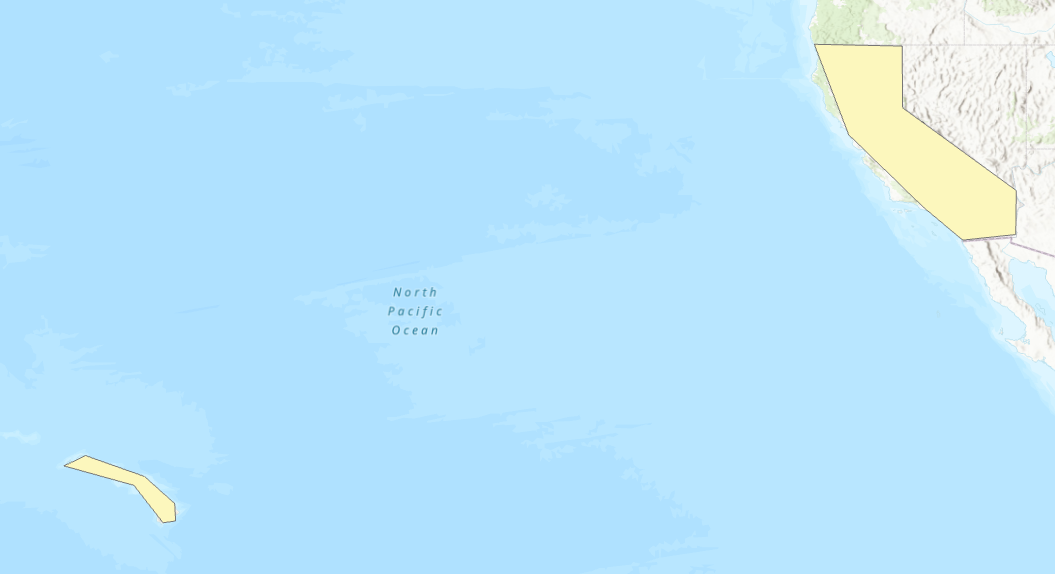
This is a single multipolygon over the Hawaii and California area. Though each part of the polygon is not too large, the extent of the multipolygon is very large containing much of the pacific ocean:
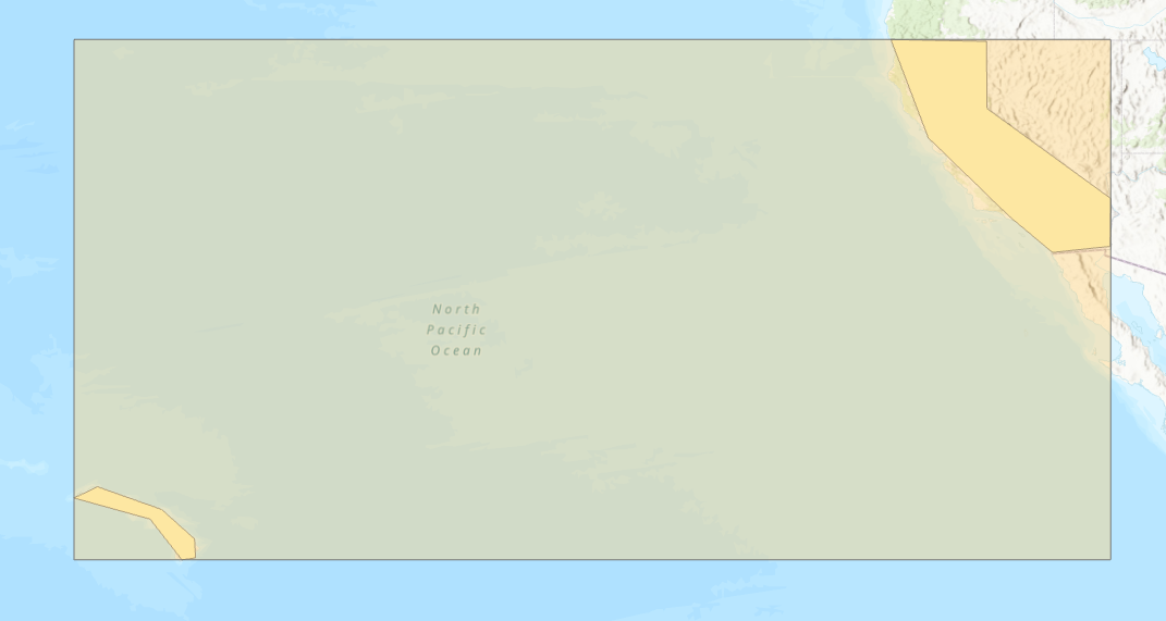
To make processing this multipolygon more efficient, use the STDump function to break it into its individual parts. Because STDump reduces the size of the extent, when BDT does its partitioning it has less to partition over.
In general, it is more efficient for BDT to process many smaller polygons than a few larger ones.
Processors as DataFrame Implicits#
Version 3.1 and above support the ability to invoke Processors as DataFrame implicits. Each Processor is now an attribute of a DataFrame, and the DataFrame is implicitly passed to the Processor when invoked. This allows processors to be chained together without intermediate variable assignment. The below example chains two Processors together:
xyDF.addShapeFromXY("X", "Y").buffer(10.0)
If the processor accepts two DataFrames as arguments, then the second must be passed to the function explicitly:
pointDF.pip(polygonDF, args*)
GeoPandas for Visualization#
The GeoPandas library can be used visualize geometries on a map embedded in a notebook. Install geopandas and its supporting libraries below into your environment:
geopandas
folium
matplotlib
mapclassify
pyarrow
If using conda/mamba, install with the following commands:
mamba install pip
pip install geopandas
mamba install -c conda-forge folium matplotlib mapclassify
mamba install pyarrow
Important Note: Using geopandas for visualization is not supported in Amazon EMR.
Ensure the spark.sql.execution.arrow.pyspark.enabled spark config is set to true.
Once installed, the BDT function to_geo_pandas() can be called on any DataFrame with a BDT Shape column to create a GeoDataFrame. This GeoDataFrame can be used to display a map with the geometries in the BDT Shape column directly in the notebook.
First import BDT and xyzservices. xyzservices is downloaded with folium and allows the use of Esri basemaps in GeoPandas visualization:
import bdt
bdt.auth("<path-to-bdt-license>")
from bdt.processors import *

import xyzservices.providers as xyz
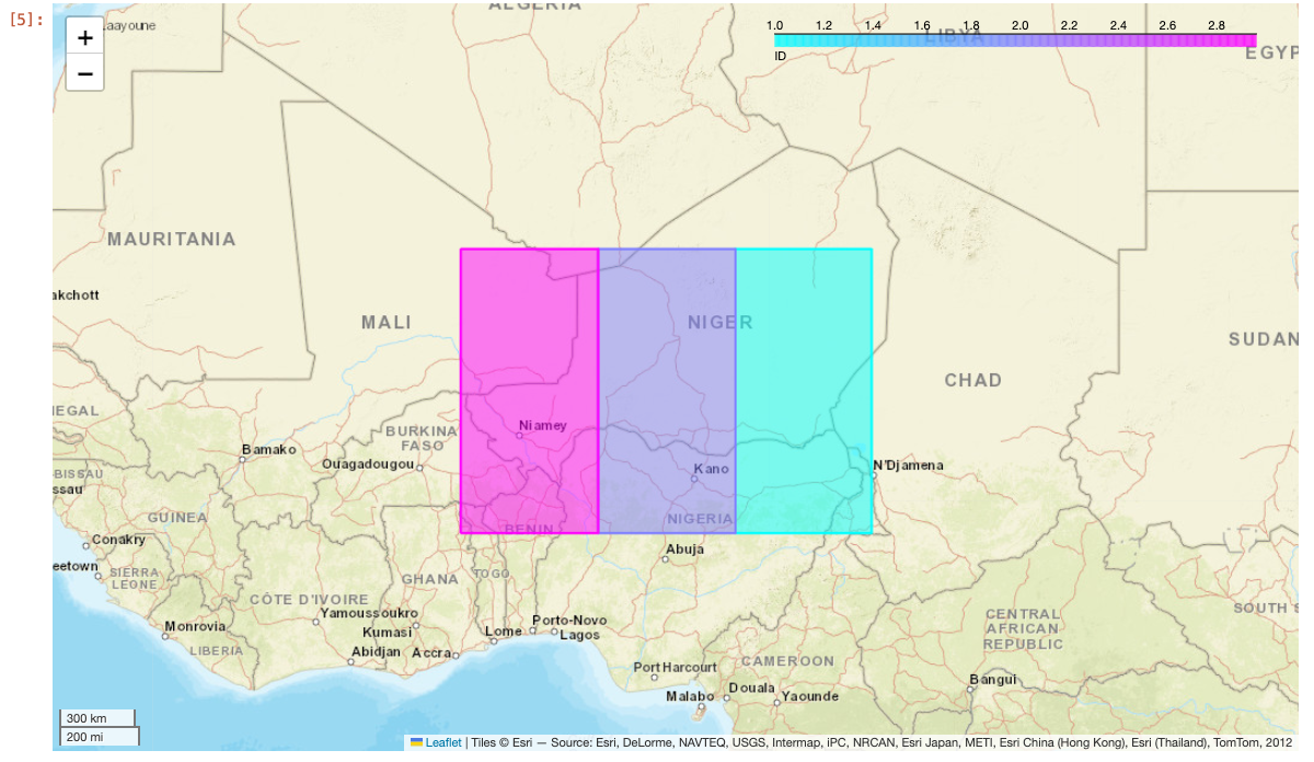
Next, call the to_geo_pandas function on any Spark DataFrame. Use the explore function on the result to display the map. To change the color of each geometry based on a column value, pass the column name into the column parameter in explore. Additionally, use the Esri World Street Map from xyzservices by passing it into the tiles parameter.
df = spark \
    .createDataFrame([(1, "POLYGON ((10 10, 15 10, 15 20, 10 20))"),
                      (2, "POLYGON ((5 10, 10 10, 10 20, 5 20))"),
                      (3, "POLYGON ((0 10, 5 10, 5 20, 0 20))")], ["ID", "WKT"]) \
    .selectExpr("ID", "ST_FromText(WKT) AS SHAPE")

gdf = df.to_geo_pandas(wkid=4326)
gdf.explore(column="ID", cmap="cool", tiles=xyz.Esri.WorldStreetMap)
Running this in a notebook cell will produce the following map:
The map can be customized further using folium. See the GeoPandas and Folium documentation for more information.
If there are multiple DataFrames that need to be displayed, consider using the to_geo_pandas_layers function. This will take a list of DataFrames, each with a shape struct column, and display them all on one map with each DataFrame on a separate layer.
df1 = spark.sql("SELECT ST_FromText('POLYGON ((10 10, 15 10, 15 20, 10 20))') SHAPE, 1 AS ID")
df2 = spark.sql("SELECT ST_FromText('POLYGON ((0 10, 5 10, 5 20, 0 20))') SHAPE, 2 AS ID")

to_geo_pandas_layers([df1, df2], 4326, ["df1", "df2"])
Running this example in a notebook cell will produce the following map:
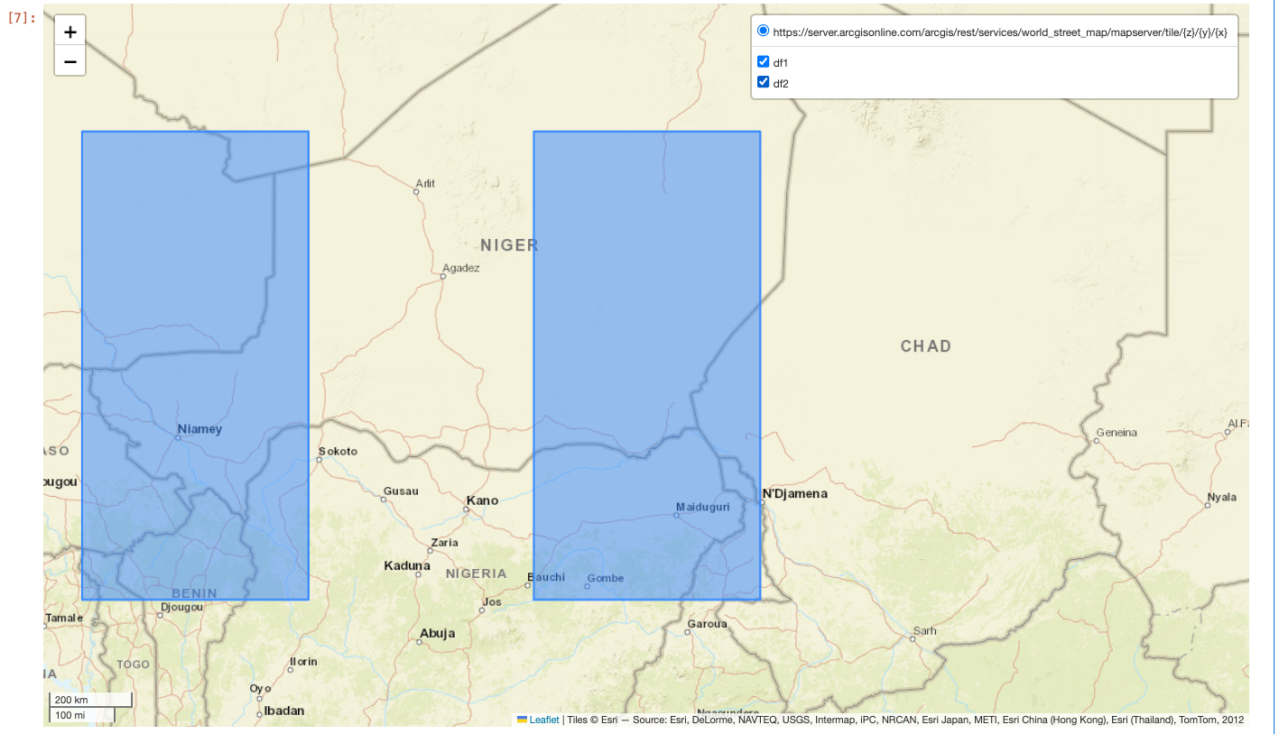
Notice the layer controls in the upper right corner of the map. This allows for toggling certain layers on and off.
to_geo_pandas_layers returns a Folium Map, so explore does not need to be called on the output.
Important Note: If the data is very large, Geopandas may not be able to visualize the entire dataset. It is best to visualize a subset of the data in this case.
Spark Broadcast Tips#
Broadcast variables enable the efficient transfer of data to all the machines in the cluster. Below are some general tips when using broadcast:
Increase the memory of each node in the cluster
Set
spark.driver.maxResultSizeto something higher (we recommend 8g)In practice, the largest dataframe that can successfully broadcast is typically 4-5 gigabytes regardless of
spark.driver.maxResultSize