Visualize H3 Binning in ArcGIS Pro#
Table of Contents#
Part 1: Overview#
This notebook will first walk through the process of acquiring raw point data and converting the points into a feature class to visualize in ArcGIS Pro. It will then show how to read the point feature class back into a Spark DataFrame, perform binning on the points based on H3 hexagons, and visulize the final results again in ArcGIS Pro.
Note: This notebook is intended to be run in an ArcGIS Pro notebook environment. Some concepts such as H3 binning can be broadly applicable but functions that convert to and from feature classes must be run in ArcGIS Pro.
[1]:
# Setup Spark for use in ArcGIS Pro

from spark_esri import spark_start, spark_stop

spark_stop()

config = {
    "spark.driver.memory":"4G",
    "spark.kryoserializer.buffer.max":"2024",
    "spark.jars": r"C:\<path-to-bdt-jar>\bdt-3.5.0-3.5.1-2.12-17.jar",
    "spark.submit.pyFiles": r"C:\<path-to-bdt-zip>\bdt-3.5.0.zip"
}

spark = spark_start(config=config)
***WARNING*** Falling back on arcgispro-py3 python.
[2]:
import bdt
from bdt import functions as B
from bdt import processors as P
from pyspark.sql.functions import count, cast, col
bdt.auth("bdt.lic")
BDT has been successfully authorized!

            Welcome to
             ___    _                ___         __             ______             __   __     _   __
            / _ )  (_)  ___ _       / _ \ ___ _ / /_ ___ _     /_  __/ ___  ___   / /  / /__  (_) / /_
           / _  | / /  / _ `/      / // // _ `// __// _ `/      / /   / _ \/ _ \ / /  /  '_/ / / / __/
          /____/ /_/   \_, /      /____/ \_,_/ \__/ \_,_/      /_/    \___/\___//_/  /_/\_\ /_/  \__/
                      /___/

BDT python version: v3.5.0-v3.5.0
BDT jar version: v3.5.0-v3.5.0
Part 2: Data Preparation#
The point data used in this notebook is AIS data from the Marine Cadastre. It can be downloaded from their website: https://marinecadastre.gov/ais/ This data comes from location transmissions from vessels in U.S. and international waters.
First, read the raw AIS data from CSV. Then filter the data to a smaller area. Finally, convert the LON and LAT values to the BDT Shape Struct.
[3]:
ais_sf = (
    spark
        .read
        .option("header", True)
        .csv(r"C:\<path-to-raw-AIS-data>\AIS_2020_01_01.csv") # Read the raw AIS data from CSV")
        .where("LON > -123.1938172 AND LON < -121.6745364 AND LAT > 37.4196147 AND LAT < 38.3495510") # Filter to SF Bay Area
        .select("MMSI",
                "LON",
                "LAT",
                B.st_makePoint("LON", "LAT").alias("SHAPE")) # Convert to BDT Shape
)

ais_sf.printSchema()
ais_sf.show()
root
 |-- MMSI: string (nullable = true)
 |-- LON: string (nullable = true)
 |-- LAT: string (nullable = true)
 |-- SHAPE: struct (nullable = true)
 |    |-- WKB: binary (nullable = true)
 |    |-- XMIN: double (nullable = true)
 |    |-- YMIN: double (nullable = true)
 |    |-- XMAX: double (nullable = true)
 |    |-- YMAX: double (nullable = true)

+---------+----------+--------+--------------------+
|     MMSI|       LON|     LAT|               SHAPE|
+---------+----------+--------+--------------------+
|367419340|-122.13640|38.04081|{[01 01 00 00 00 ...|
|538004188|-122.34710|37.75965|{[01 01 00 00 00 ...|
|477542400|-122.35415|37.76973|{[01 01 00 00 00 ...|
|366831930|-122.39350|37.79683|{[01 01 00 00 00 ...|
|367122220|-122.34234|37.80515|{[01 01 00 00 00 ...|
|367143460|-122.39450|37.79791|{[01 01 00 00 00 ...|
|367349770|-122.39588|37.86992|{[01 01 00 00 00 ...|
|367155780|-122.27717|37.79149|{[01 01 00 00 00 ...|
|366989360|-122.29194|38.05335|{[01 01 00 00 00 ...|
|256186000|-122.26087|38.05695|{[01 01 00 00 00 ...|
|367795270|-122.44374|37.87241|{[01 01 00 00 00 ...|
|369567000|-122.36029|37.79402|{[01 01 00 00 00 ...|
|366798310|-122.68777|37.77810|{[01 01 00 00 00 ...|
|367396710|-122.31838|37.79657|{[01 01 00 00 00 ...|
|371752000|-122.72802|37.47383|{[01 01 00 00 00 ...|
|367533950|-122.40758|37.80836|{[01 01 00 00 00 ...|
|367401030|-122.26302|38.05696|{[01 01 00 00 00 ...|
|367389840|-122.02348|38.05917|{[01 01 00 00 00 ...|
|366970020|-122.50852|37.94411|{[01 01 00 00 00 ...|
|366862680|-122.33940|37.74013|{[01 01 00 00 00 ...|
+---------+----------+--------+--------------------+
only showing top 20 rows
Part 3: Visualize Point Data#
Utilize the
to_feature_classBDT processor to save the filtered down AIS data to a feature class in the scratch workspace in ArcGIS Pro.Note: The
to_feature_classfunction will only work in an ArcGIS Pro notebook
[4]:
P.to_feature_class(ais_sf,
                   feature_class_name="AIS_SF",
                   wkid=4326,
                   workspace="scratch",
                   shape_field="SHAPE")
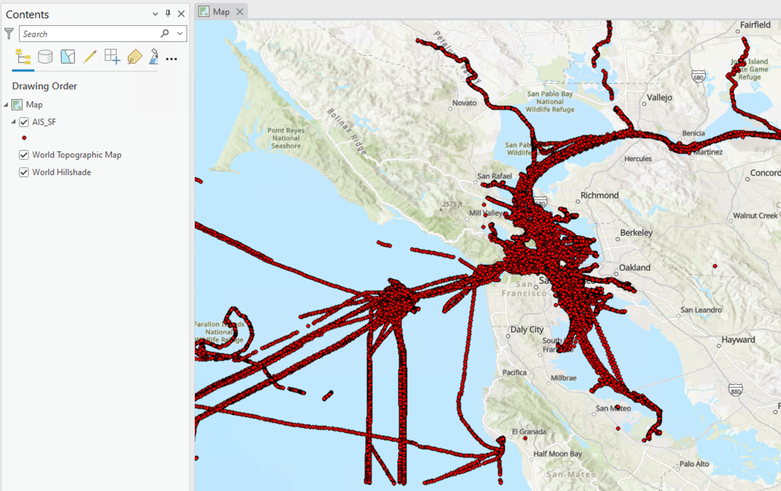
Looking at the Map in ArcGIS Pro, the point data is visualized.
Part 4: Bin Points Into H3 Hexes#
Next, utilize the
from_feature_classBDT processor to convert the feature class created in the last step back to a Spark DataFrame for H3 binning.
from_feature_classreturns the geometry column in WKB format, convert the WKB to the BDT Shape Struct withst_fromWKB.
[5]:
df = P.from_feature_class("AIS_SF")
df = df.withColumn("SHAPE", B.st_fromWKB("Shape"))

df.printSchema()
df.show()
root
 |-- OBJECTID: long (nullable = true)
 |-- SHAPE: struct (nullable = true)
 |    |-- WKB: binary (nullable = true)
 |    |-- XMIN: double (nullable = true)
 |    |-- YMIN: double (nullable = true)
 |    |-- XMAX: double (nullable = true)
 |    |-- YMAX: double (nullable = true)
 |-- MMSI: string (nullable = true)
 |-- LON: string (nullable = true)
 |-- LAT: string (nullable = true)

+--------+--------------------+---------+----------+--------+
|OBJECTID|               SHAPE|     MMSI|       LON|     LAT|
+--------+--------------------+---------+----------+--------+
|       1|{[01 01 00 00 00 ...|367419340|-122.13640|38.04081|
|       2|{[01 01 00 00 00 ...|538004188|-122.34710|37.75965|
|       3|{[01 01 00 00 00 ...|477542400|-122.35415|37.76973|
|       4|{[01 01 00 00 00 ...|366831930|-122.39350|37.79683|
|       5|{[01 01 00 00 00 ...|367122220|-122.34234|37.80515|
|       6|{[01 01 00 00 00 ...|367143460|-122.39450|37.79791|
|       7|{[01 01 00 00 00 ...|367349770|-122.39588|37.86992|
|       8|{[01 01 00 00 00 ...|367155780|-122.27717|37.79149|
|       9|{[01 01 00 00 00 ...|366989360|-122.29194|38.05335|
|      10|{[01 01 00 00 00 ...|256186000|-122.26087|38.05695|
|      11|{[01 01 00 00 00 ...|367795270|-122.44374|37.87241|
|      12|{[01 01 00 00 00 ...|369567000|-122.36029|37.79402|
|      13|{[01 01 00 00 00 ...|366798310|-122.68777|37.77810|
|      14|{[01 01 00 00 00 ...|367396710|-122.31838|37.79657|
|      15|{[01 01 00 00 00 ...|371752000|-122.72802|37.47383|
|      16|{[01 01 00 00 00 ...|367533950|-122.40758|37.80836|
|      17|{[01 01 00 00 00 ...|367401030|-122.26302|38.05696|
|      18|{[01 01 00 00 00 ...|367389840|-122.02348|38.05917|
|      19|{[01 01 00 00 00 ...|366970020|-122.50852|37.94411|
|      20|{[01 01 00 00 00 ...|366862680|-122.33940|37.74013|
+--------+--------------------+---------+----------+--------+
only showing top 20 rows
Bin the data by H3 Hexagon:
Assign each point its H3 Index with
geoToH3.Group by the H3 Index to group together all points in the same H3 hexagon.
Use
countto aggregate the number of points in each hexagon.Construct the H3 Hexagon geometry from the H3 Index with
h3ToGeoBoundaryandst_makePolygon.
[6]:
binned = (
    df
        .withColumn("H3_IDX", B.geoToH3("SHAPE.YMIN", "SHAPE.XMIN", 8)) # Get the H3 Index for each point at H3 resolution 8
        .groupBy("H3_IDX") # Group points in the same H3 hexagon
        .agg(
            count("*").alias("COUNT"), # Aggregate the number of points in each Hexagon
        )
        .withColumn("SHAPE", B.st_makePolygon(B.h3ToGeoBoundary("H3_IDX"))) # Convert from H3 Index to hexagon geometry
)

binned.printSchema()
binned.show()
root
 |-- H3_IDX: long (nullable = true)
 |-- COUNT: long (nullable = false)
 |-- SHAPE: struct (nullable = true)
 |    |-- WKB: binary (nullable = true)
 |    |-- XMIN: double (nullable = true)
 |    |-- YMIN: double (nullable = true)
 |    |-- XMAX: double (nullable = true)
 |    |-- YMAX: double (nullable = true)

+------------------+-----+--------------------+
|            H3_IDX|COUNT|               SHAPE|
+------------------+-----+--------------------+
|613196571586068479|   61|{[01 06 00 00 00 ...|
|613196571579777023|   62|{[01 06 00 00 00 ...|
|613196569748963327|   57|{[01 06 00 00 00 ...|
|613196903001096191|    7|{[01 06 00 00 00 ...|
|613196902925598719|   11|{[01 06 00 00 00 ...|
|613196911291138047|    7|{[01 06 00 00 00 ...|
|613196569702825983|  613|{[01 06 00 00 00 ...|
|613196541582114815|   49|{[01 06 00 00 00 ...|
|613196571193901055|   60|{[01 06 00 00 00 ...|
|613196820266352639|    9|{[01 06 00 00 00 ...|
|613196571550416895|   64|{[01 06 00 00 00 ...|
|613196572957605887|  565|{[01 06 00 00 00 ...|
|613196569721700351|  541|{[01 06 00 00 00 ...|
|613196569774129151|   15|{[01 06 00 00 00 ...|
|613196573045686271|   30|{[01 06 00 00 00 ...|
|613196539975696383|  483|{[01 06 00 00 00 ...|
|613196904959836159|    8|{[01 06 00 00 00 ...|
|613196539826798591|   92|{[01 06 00 00 00 ...|
|613196898311864319|    3|{[01 06 00 00 00 ...|
|613196899435937791|    8|{[01 06 00 00 00 ...|
+------------------+-----+--------------------+
only showing top 20 rows
Part 5: Visualize Bins#
Before visualization, cast the
H3_IDXto string. This must be done since ArcGIS Pro does not support storing Long values over 53 bits and most H3 indexes are over 53 bits.Then, utilize the
to_feature_classBDT processor again to save the H3 binned AIS data to a feature class in the scratch workspace in ArcGIS Pro.
[7]:
P.to_feature_class(binned.select(col("H3_IDX").cast("string"), "COUNT", "SHAPE"), # Pro only supports up to 53 bit longs
                   feature_class_name="AIS_BINNED",
                   wkid=4326,
                   workspace="scratch",
                   shape_field="SHAPE")
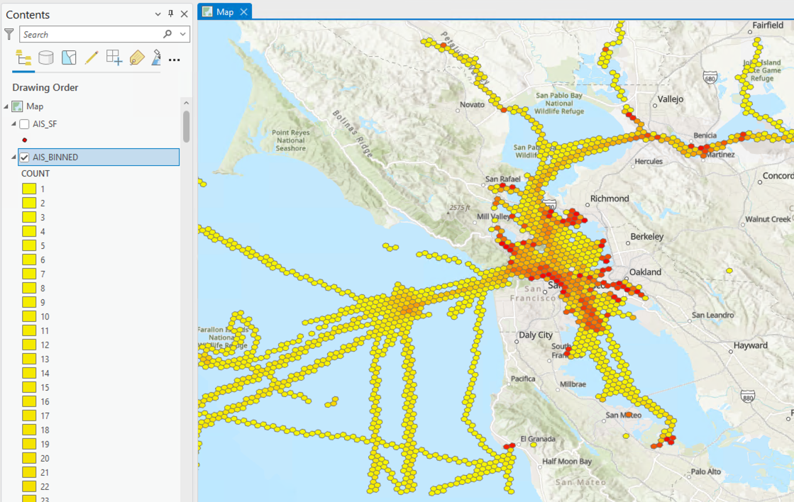
In ArcGIS Pro, the symbology color can be customized to reflect the number of points binned into each hexagon. The result is a heat map of vessel activity in the San Francisco bay area.